Amplitude Analyses of D →πππ
Welcome
Welcome to the webpage dedicated to the D → πππ amplitude analyses. The analyses is being performed with LHCb data collected in 2012 whose total recorded luminosity writen to disk is approx. (1988 ∓ 23.86)/fb. Those data have about 70 millions events.
MVA studies
In Boosted Decision Trees, the selection is done on a majority vote on the result of several decision trees, which are all derived from the same training sample by supplying different event weights during the training.
Decision Trees: successive decision nodes are used to categorize the events out of the sample as either signal or background. Each node uses only a single discriminating variable to decide if the event is signal-like ("goes right") or background-like ("goes left"). This forms a tree like structure with "baskets" at the end (leave nodes), and an event is classified as either signal or background according to whether the basket where it ends up has been classified signal or background during the training. Training of a decision tree is the process to define the "cut criteria" for each node. The training starts with the root node. Here one takes the full training event sample and selects the variable and corresponding cut value that gives the best separation between signal and background at this stage. Using this cut criterion, the sample is then divided into two subsamples, a signal-like (right) and a background-like (left) sample. Two new nodes are then created for each of the two sub-samples and they are constructed using the same mechanism as described for the root node. The devision is stopped once a certain node has reached either a minimum number of events, or a minimum or maximum signal purity. These leave nodes are then called "signal" or "background" if they contain more signal respective background events from the training sample.
Boosting: the idea behind the boosting is, that signal events from the training sample, that end up in a background node (and vice versa) are given a larger weight than events that are in the correct leave node. This results in a re-weighed training event sample, with which then a new decision tree can be developed. The boosting can be applied several times (typically 100-500 times) and one ends up with a set of decision trees (a forest).
Analysis: applying an individual decision tree to a test event results in a classification of the event as either signal or background. For the boosted decision tree selection, an event is successively subjected to the whole set of decision trees and depending on how often it is classified as signal, a "likelihood" estimator is constructed for the event being signal or background. The value of this estimator is the one which is then used to select the events from an event sample, and the cut value on this estimator defines the efficiency and purity of the selection.
Official MTVA page here.
Test 0
The first test were performed with 15 variables:
- D_IP_OWNPV
- D_IPCHI2_OWNPV
- D_FD_OWNPV
- D_FDCHI2_OWNPV
- D_DIRA_OWNPV
- D_ENDVERTEX_CHI2
- D_DOCA12
- D_DOCA13
- D_DOCA23
- PTsum
- logIP
- D_BPVTRGPOINTING
- p1_IPCHI2_OWNPV
- p2_IPCHI2_OWNPV
- p3_IPCHI2_OWNPV
- NSpec 1
- D_MM (spectator)
Training sample: MC signal with TRUEID for D+ and its daughters. The weight of the signal is the PIDCalib variable called D_PIDEff. Background sample have 500000 events made from the right side wing (D_MM:(1910, 1930)) from data . No cut is applied to the background sample, no PID, no IP, etc..... This test is run over 10000 entries for signal and background. The classifiers tested were:
- mva_BDT
- mva_FDA_GA
- mva_KNN
- mva_LD
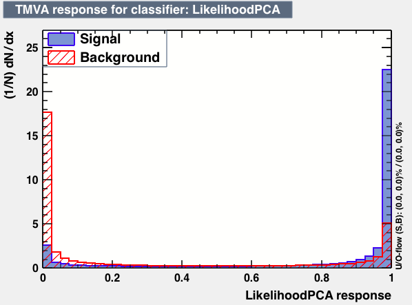
- mva_Likelihood
- mva_LikelihoodPCA
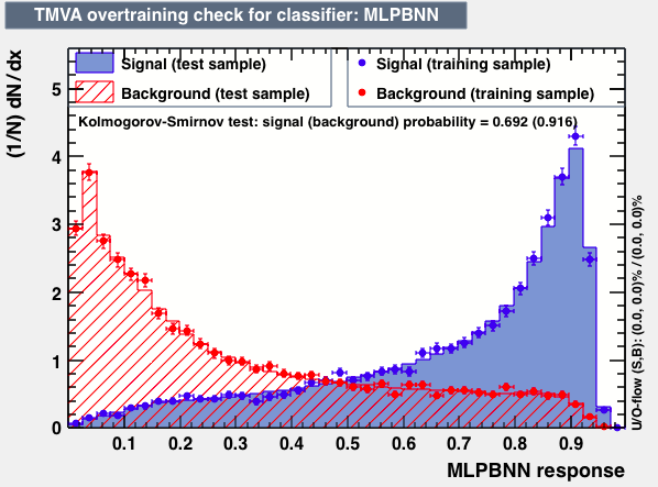
- mva_MLPBNN
- mva_PDEFoamBoost
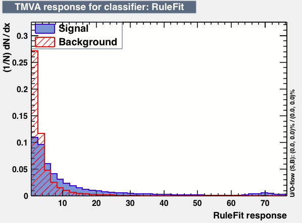
- mva_RuleFit
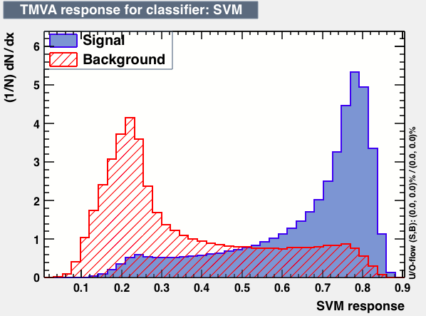
- mva_SVM
Below are some results:
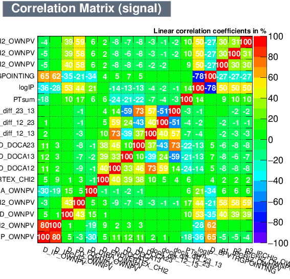
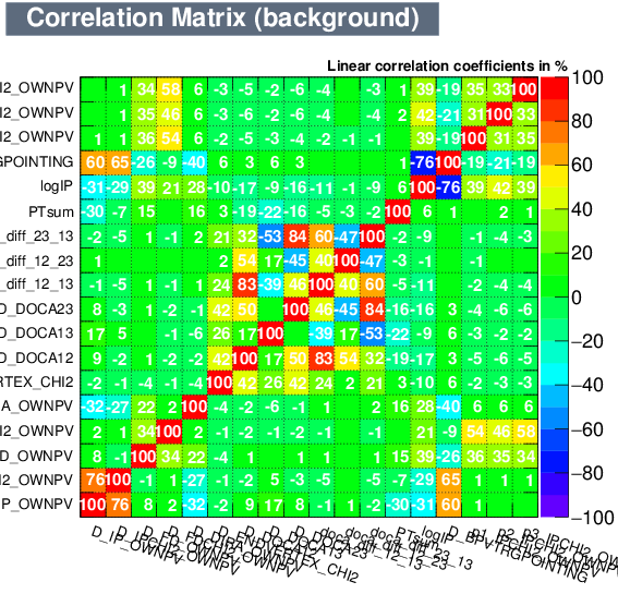
| Correlation matrix | |
|---|---|
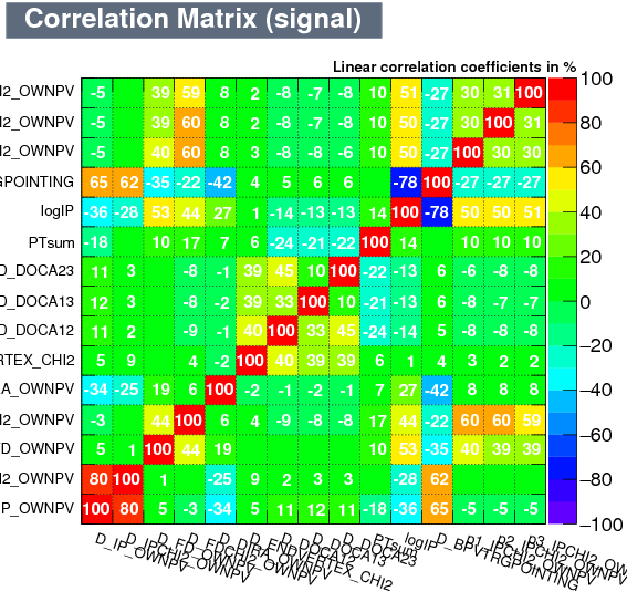
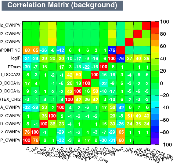
| Signal | Background |
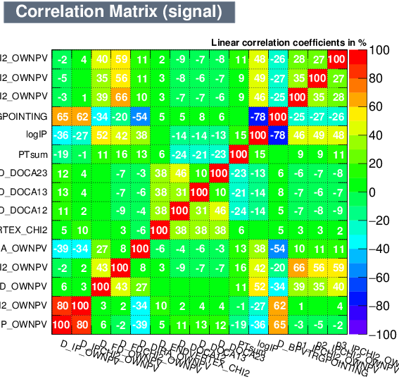 |
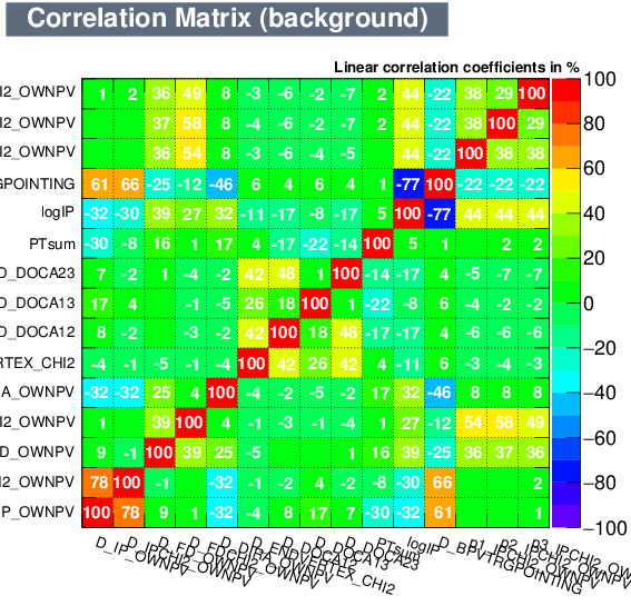 |
| Rejection Background vs Signal efficiency |
|---|
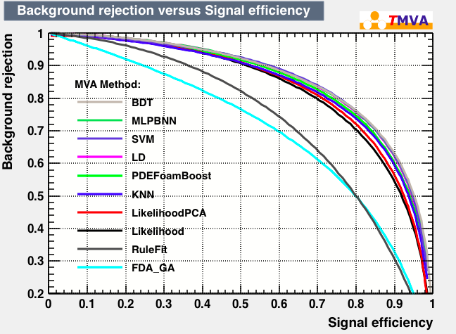 |
| Classifiers | |||
|---|---|---|---|
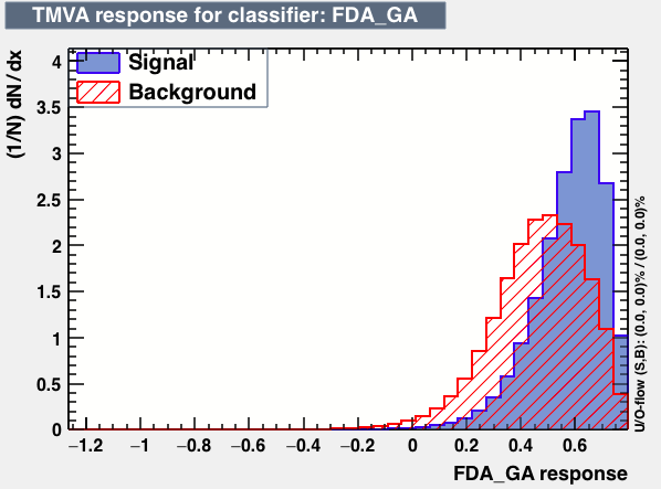
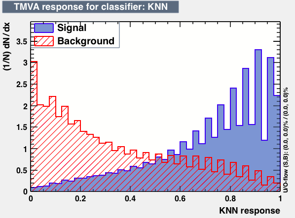
| Parameter | BDT | FDA_GA | KNN |
| Output | 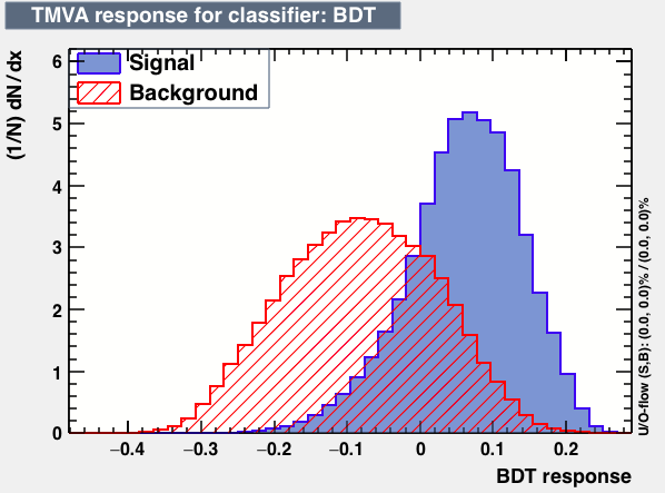 |
 |
 |
| Efficiencies | 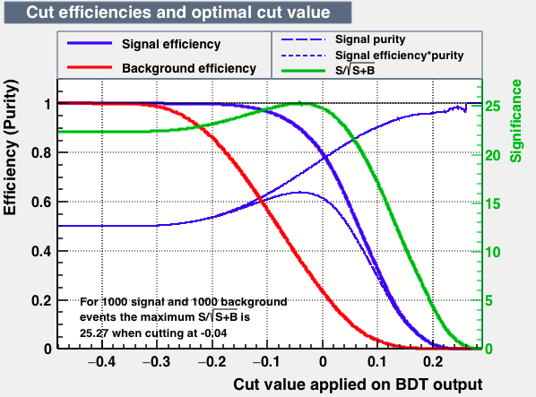 |
 |
 |
| Overtrain | 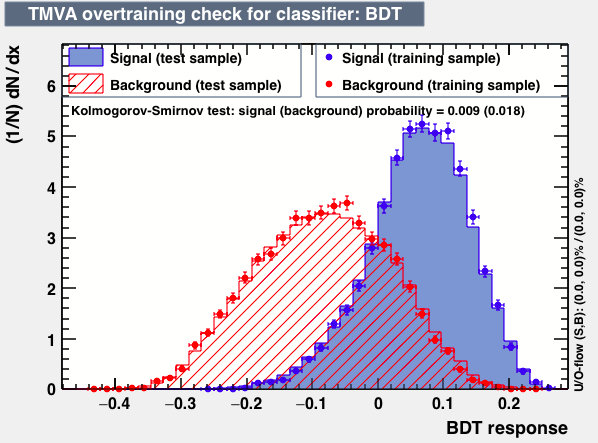 |
 |
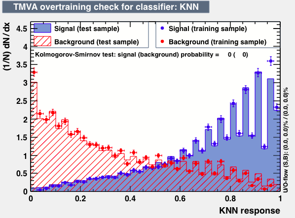 |
| Classifiers | |||
|---|---|---|---|
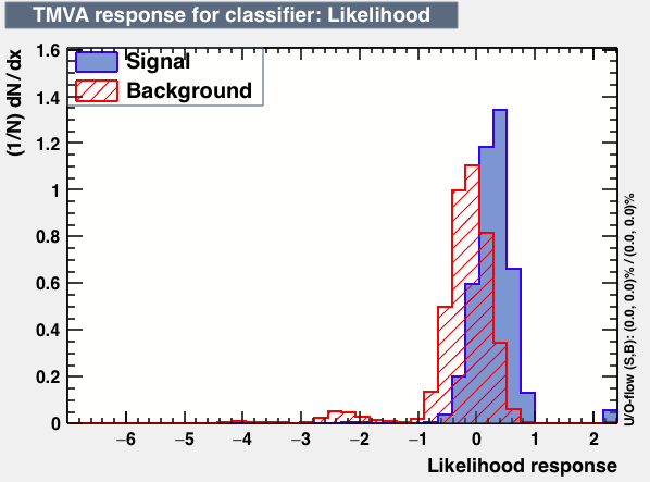
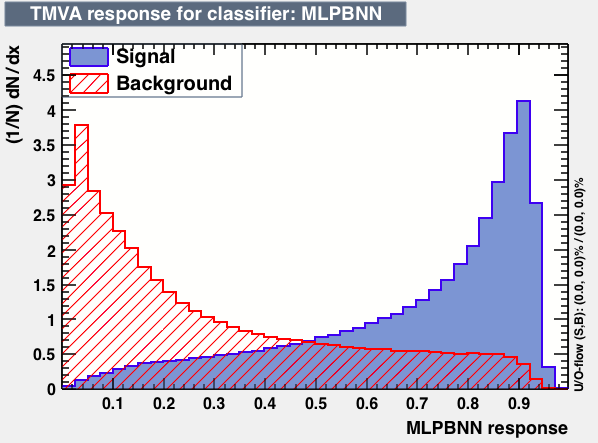
| Parameter | LD | Likelihood | MLPBNN |
| Output | 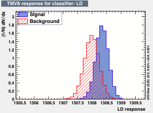 |
 |
 |
| Efficiencies | 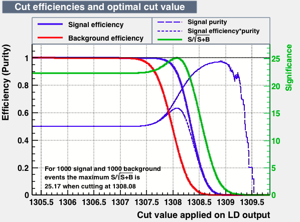 |
 |
 |
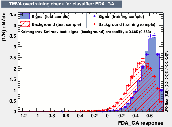
| Overtrain | 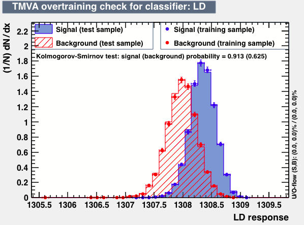 |
 |
 |
| Classifiers | |||
|---|---|---|---|
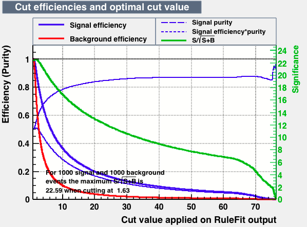
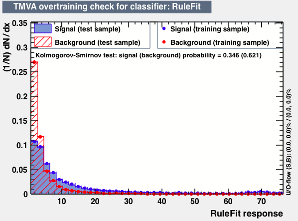
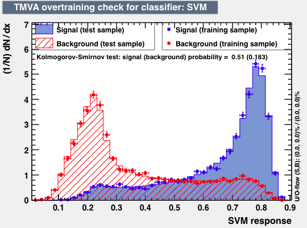
| Parameter | PDEFoamBoost | RuleFit | SVM |
| Output | 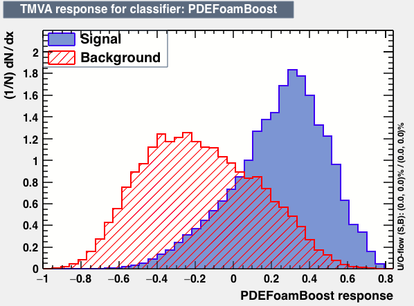 |
 |
 |
| Efficiencies | 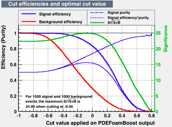 |
 |
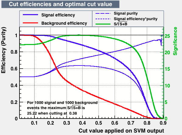 |
| Overtrain | 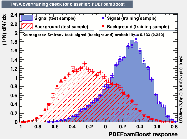 |
 |
 |
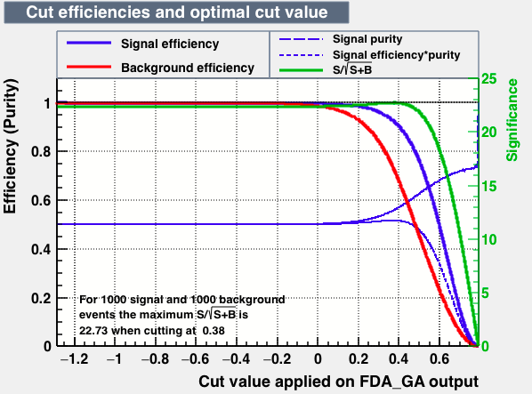
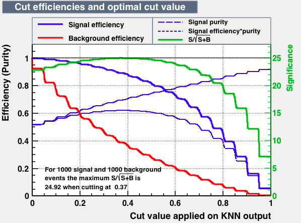
Conclusions of test0
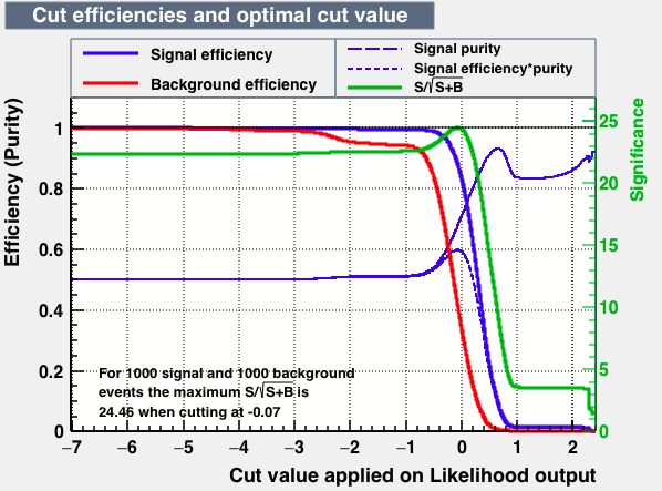
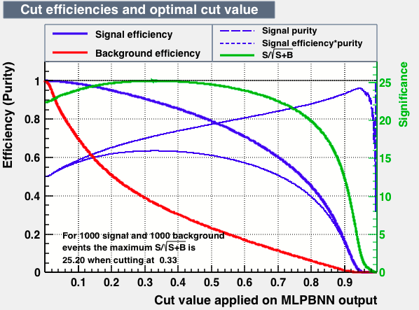
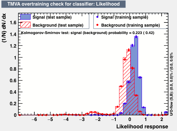
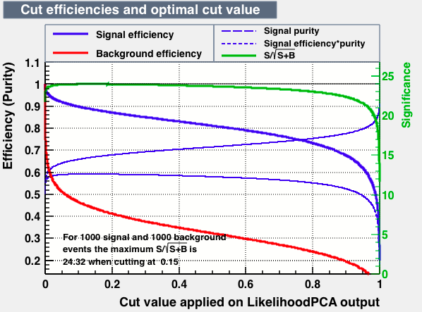
From this first test one may conclude the best candidates classifiers for MVA are: BDT, MLPBNN, KNN and SVM:
| Best Candidates | ||||
|---|---|---|---|---|
| BDT | MLPBNN | KNN | SVM | |
| S/sqrt(S + B) | 25.27 | 25.20 | 24.92 | 25.22 | Cut | -0.04 | 0.33 | 0.37 | 0.38 |
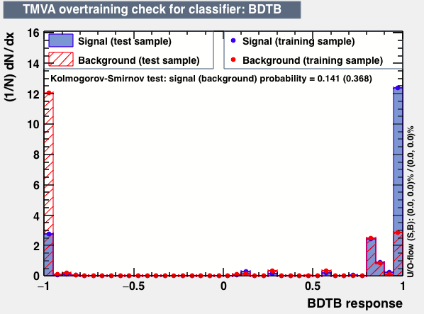
P.S: BDT KS-test have very small probabilities which may be due to overtraining. In this test the training and testing samples have very different number of entries.
Test 1
The second test were performed with 18 variables:
- D_IP_OWNPV
- D_IPCHI2_OWNPV
- D_FD_OWNPV
- D_FDCHI2_OWNPV
- D_DIRA_OWNPV
- D_ENDVERTEX_CHI2
- D_DOCA12
- D_DOCA13
- D_DOCA23
- doca_diff_12_13 = D_DOCA12 - D_DOCA13
- doca_diff_12_23 = D_DOCA12 - D_DOCA23
- doca_diff_23_13 = D_DOCA23 - D_DOCA13
- PTsum
- logIP
- D_BPVTRGPOINTING
- p1_IPCHI2_OWNPV
- p2_IPCHI2_OWNPV
- p3_IPCHI2_OWNPV
Training samples for signal and background are the same that of the Test 1 apart number of training events. Training with 250000 entries for signal and MC. The classifiers tested were:
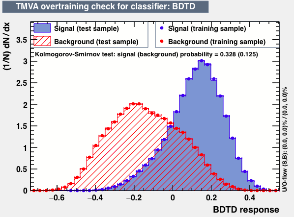
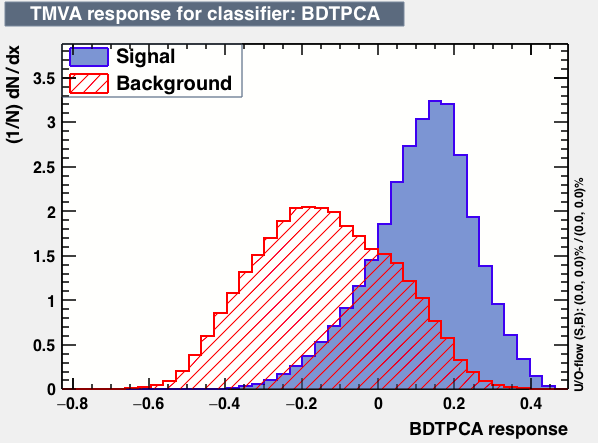
- mva_BDT
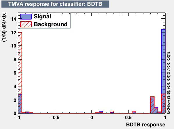
- mva_BDTB
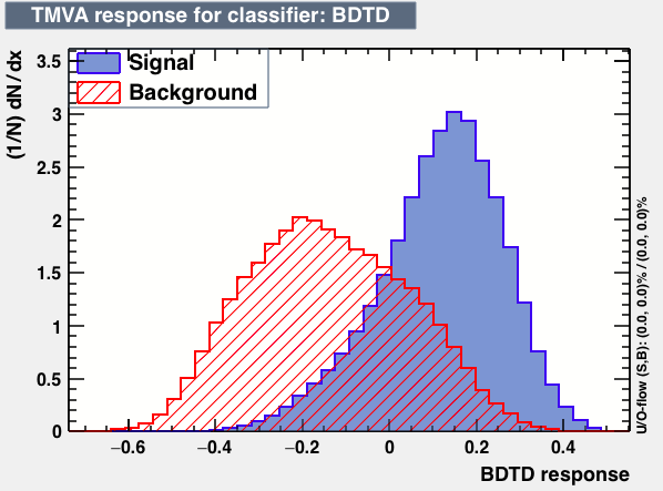
- mva_BDTD
- mva_BDTG
- mva_BDTPCA
- mva_LikelihoodPCA
- mva_RuleFit
Bellow some results:
| Correlation matrix | |
|---|---|
| Signal | Background |
 |
 |
| Rejection Background vs Signal efficiency |
|---|
 |
| Classifiers | |||
|---|---|---|---|
| Parameter | BDT | BDTB | BDTD |
| Output | 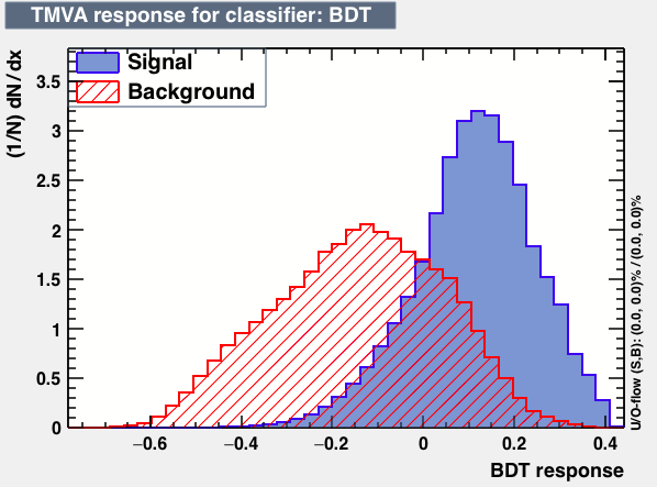 |
 |
 |
| Efficiencies | 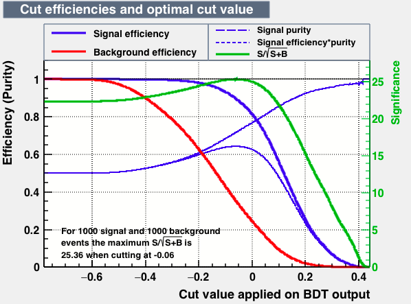 |
 |
 |
| Overtrain | 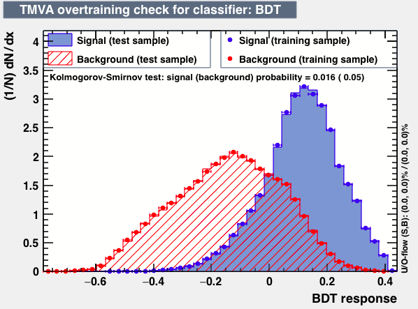 |
 |
 |
| Classifiers | |||
|---|---|---|---|
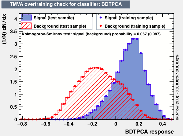
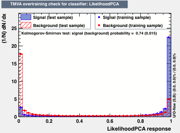
| Parameter | BDTG | BDTPCA | LikelihoodPCA |
| Output | 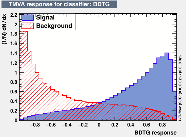 |
 |
 |
| Efficiencies | 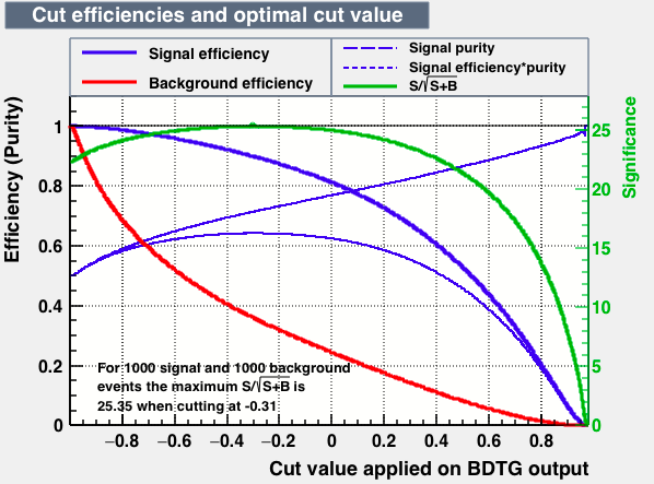 |
 |
 |
| Overtrain | 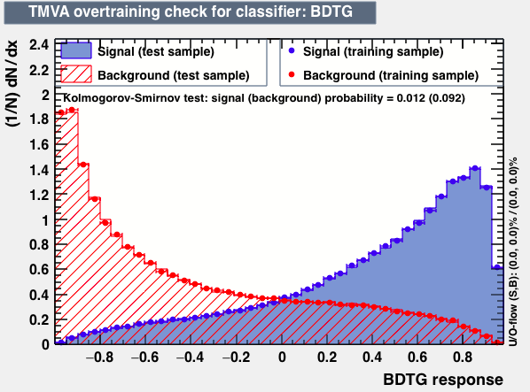 |
 |
 |
| Classifiers | |
|---|---|
| Parameter | mva_RuleFit |
| Output | 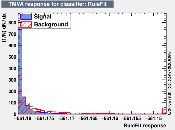 |
| Efficiencies | 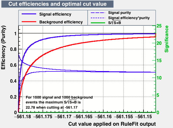 |
| Overtrain | 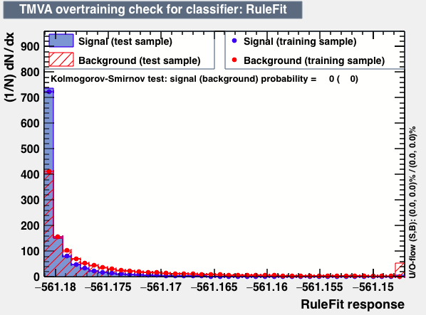 |
Conclusions of test1
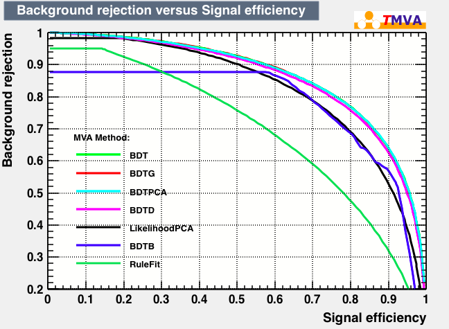
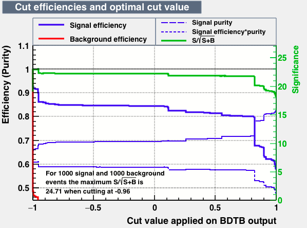
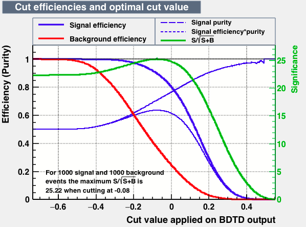
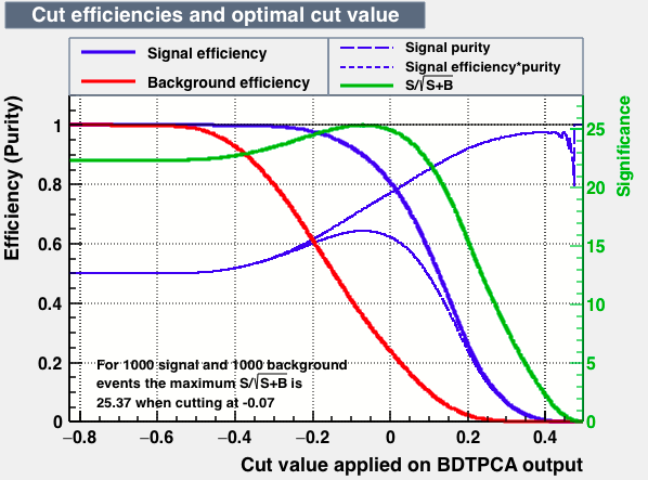
As expected from the first test (test0) the best candidates for the classifiers are BDT and BDTPCA. BDTPCA is the BDT but with the input variables transformed over a PCA-transformation. PCA is a linear transformation that rotates a sample of data points such that the maximum variability is visible. It thus identifies the most important gradients. In the PCA-transformed coordinate system, the largest variance by any projection of the data comes to lie on the first coordinate (denoted the first principal component), the second largest variance on the second coordinate, and so on.
| Best Candidates | ||
|---|---|---|
| BDT | BDTPCA | |
| S/sqrt(S + B) | 25.36 | 25.37 | Cut | -0.06 | -0.07 | Signal K-S test | 0.016 | 0.067 | Bkg K-S test | 0.05 | 0.087 |
Again the number of training and test samples differs largely. The training sample for both signal and background was of 250000. The Test samples for signal was of 1831874 while for background was of 250000. For the next test we uniform the number of events of background to the maximum avaliable statistic in the signal from MC samples. The MC sample for MagUp + magDown with trueID for D and its daughters have 2081874 simulated events. Therefore we make a background sample from data with the same amount of events that of signal MC (2081874).
Test 2
The Third test were performed with 15 variables:
- D_IP_OWNPV
- D_IPCHI2_OWNPV
- D_FD_OWNPV
- D_FDCHI2_OWNPV
- D_DIRA_OWNPV
- D_ENDVERTEX_CHI2
- D_DOCA12
- D_DOCA13
- D_DOCA23
- PTsum
- logIP
- D_BPVTRGPOINTING
- p1_IPCHI2_OWNPV
- p2_IPCHI2_OWNPV
- p3_IPCHI2_OWNPV
Training samples for signal and background are the same that of the Test 1 apart number of training events. In total 1040937 signal and background events was used for training and test of the two MVA tested. The classifiers tested were:
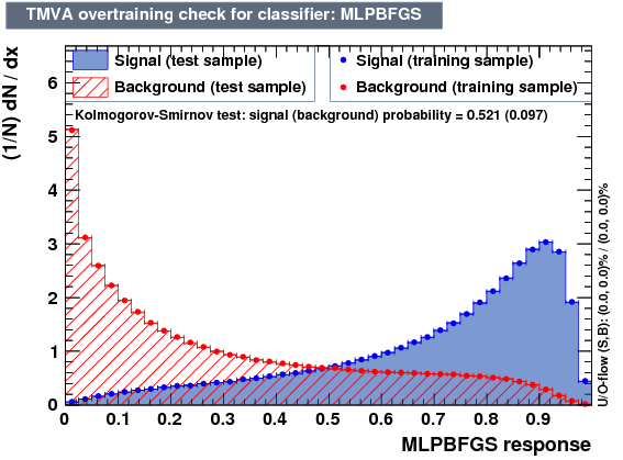
- mva_BDTPCA
- mva_MLPBFGS
MLPBFGS is recommended Artificial Neural Networks (Non-Linear Discriminant Analysis - ANN) with optional training method. The MLP method is very similar to the ROOT ANN, but can be trained significantly faster. The input layer contains as many neurons as input variables used in the MVA. The output layer contains a single neuron for the signal weight. In between the input and output layers are a variable number of k hidden layers with arbitrary numbers of neurons. (While the structure of the input and output layers is determined by the problem, the hidden layers can be configured by the user through the option string of the method booking.)
Bellow some results:
| Correlation matrix | |
|---|---|
| Signal | Background |
 |
 |
| Rejection Background vs Signal efficiency |
|---|
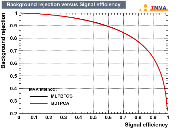 |
| Classifiers | ||
|---|---|---|
| Parameter | BDTPCA | MLPBFGS |
| Output | 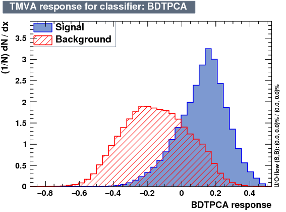 |
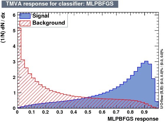 |
| Efficiencies | 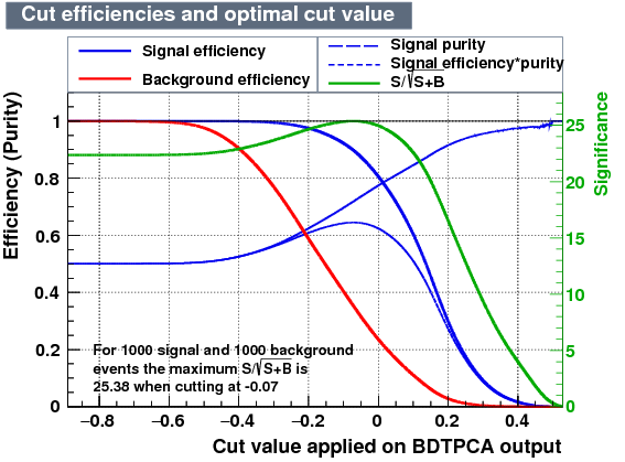 |
 |
| Overtrain | 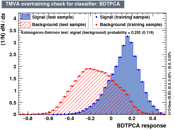 |
 |
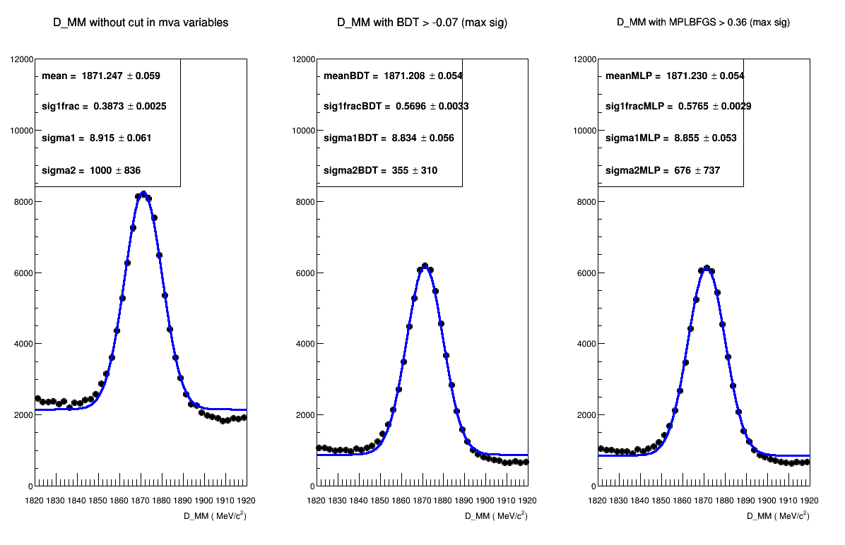
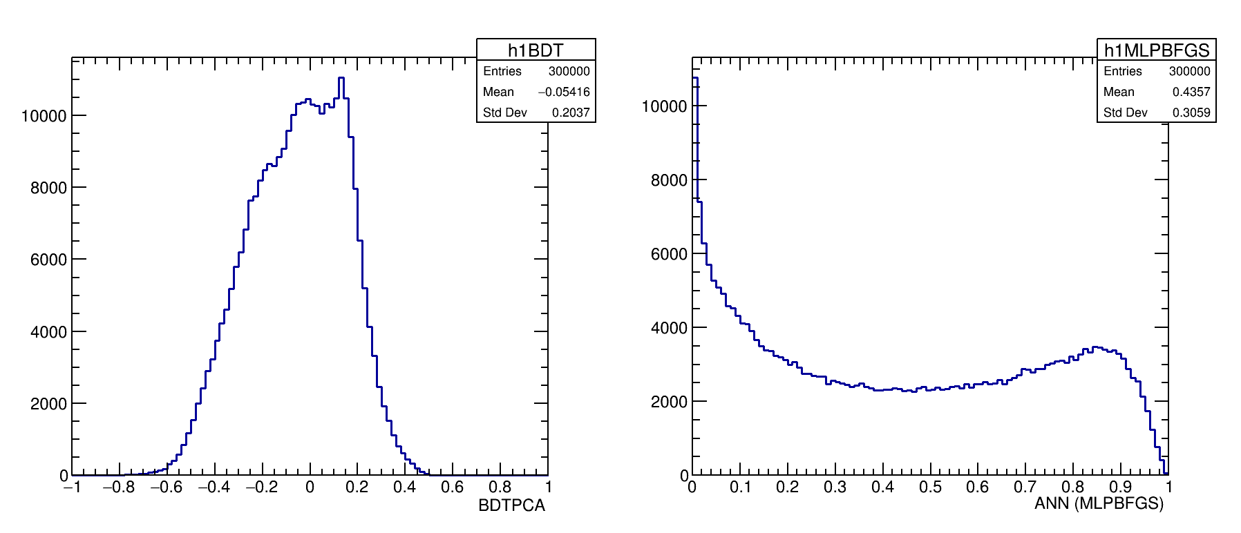
Application
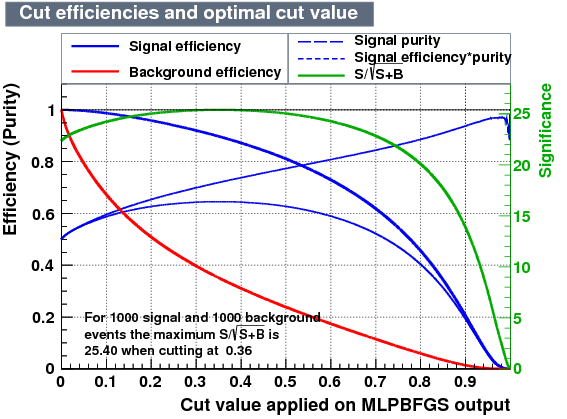
From the efficiency plots above we account for the retention of events from data in the window:
- Retention of events BDTPCA = 41.59 %
- Retention of events MLPBFGS = 42.38 %
Mass plot bellow (300k events):
MVA responses on data
TMVA update
The above TMVA studies can not be applied for amplitude analyses once any cut on the variables pi_IPCHI2_OWNPV is know to distort the DP (font, Josué Thesys). The varibles for training have to carry information from the topology of the event, specially of the mother particle.
From the above studies one can conclude that neither the mva_FDA_GA, the linelar discriminator LD and LikelihoodPCA and nor the ANN based training have better discrimination power than the BDT.
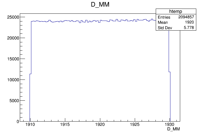
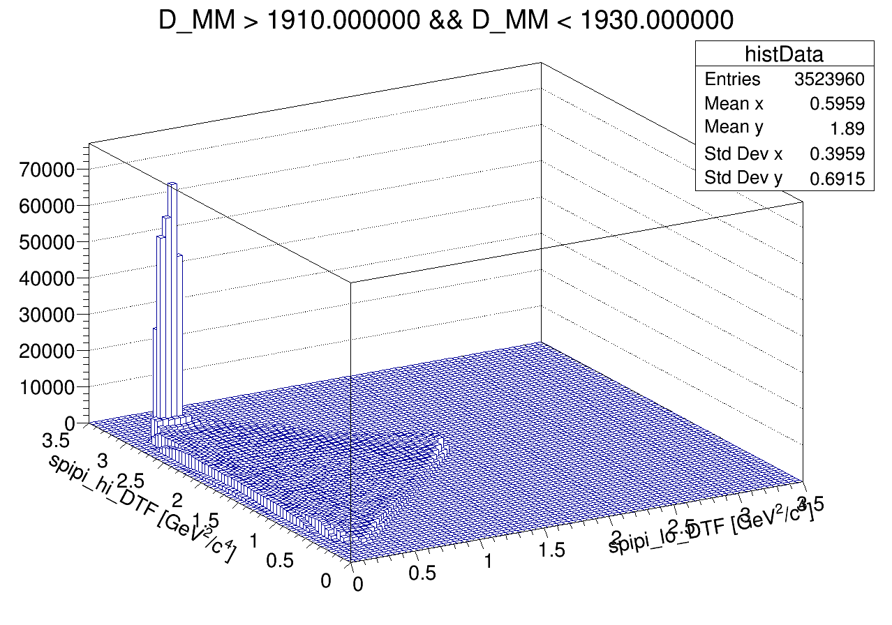
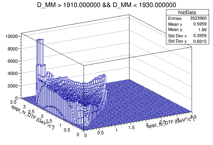
The improvement from previous studies is the correction on the signal selection with BKG_CAT == 0 || BKG_CAT == 50 for the signal selection. The sinal sample have in total 2094857 simulated events fully reconstructed with the LHCb software framework. Those data also have the magneto UP and Down selection with about 50% each. The background sample is composed of events populating the right wing of the invariant mass distribution, between 1910 and 1930 MeV. The sample have 85% magneto Down events and 15 % magneto Up due to the method of merge the magUp and magDown sample: first the sample was merged and then cut on the first 2094857 events to account for the same number of entries availiable in the MC sample.
The test is done with 12 variables:- D_IP_OWNPV"
- D_IPCHI2_OWNPV"
- D_FD_OWNPV"
- D_FDCHI2_OWNPV"
- D_DIRA_OWNPV"
- D_ENDVERTEX_CHI2"
- doca_diff_12_13 := D_DOCA12 - D_DOCA13
- doca_diff_12_23 := D_DOCA12 - D_DOCA23
- doca_diff_23_13 := D_DOCA23 - D_DOCA13
- PTsum
- logIP
- D_BPVTRGPOINTING
Training sample: MC signal with BKG_CAT == 0 || BKG_CAT ==50. The weight of the signal is the PIDCalib variable called D_PIDEff. Background sample have 2094857 events made from the right side wing (D_MM:(1910, 1930)) from data. No cut is applied to the background sample, no PID, no IP, etc..... The classifiers tested were:
- mva_BDTPCA
- mva_MLPBFGS
| BDTPCA | |
|---|---|
| Parameter | Value |
| Number of trees | 1000 |
| MinNodeSize | 2.5% |
| MaxDepth | 3 |
| BoostType | AdaBoost |
| AdaBoostBeta | 0.5 |
| UseBaggedBoost | --- |
| BaggedSampleFraction | 0.5 |
| SeparationType | GiniIndex |
| nCuts | 20 |
| VarTransform | PCA |
| MLPBFGS | |
|---|---|
| Parameter | Value |
| NeuronType | tanh |
| VarTransform | N |
| NCycles | 600 |
| HiddenLayers | N+5 |
| TestRate | 5 |
| TrainingMethod | BFGS |
| UseRegulator | No |
Selection
Below you can find the current status of the analysis with a new BDT selection, 1D mass fit with expected purity and Dalitz plots.
TMVA (test7)
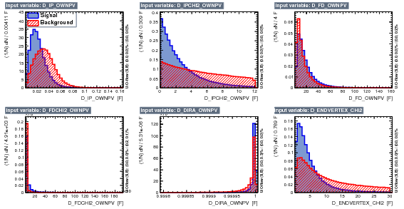
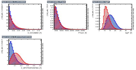
As discussed above the TMVA was updated by removing the pi_IPCHI2_OWNPV variables and complementary, in this version, we include a D_DOCAMAX which is the maximum distance of approach between pairs of tracks, i.e, maximum values between D_DOCA12, D_DOCA23 and D_DOCA13. Therefore this BDT version have in total 10 input variables:
- D_IP_OWNPV
- D_IPCHI2_OWNPV
- D_FD_OWNPV
- D_FDCHI2_OWNPV
- D_DIRA_OWNPV
- D_ENDVERTEX_CHI2
- D_DOCAMAX
- PTsum
- logIP
- D_BPVTRGPOINTING
The BDT discriminator is the used alone, which is trained with 2094857 signal events from 2012 MC sample (the old sample). This sample is made with BKG_CAT == 0 || BKG_CAT == 50 for the signal selection. Those selection also have the magnet UP and Down with about 50% each. During the training the signal weight D_PIDEff from PIDCalib is applied.
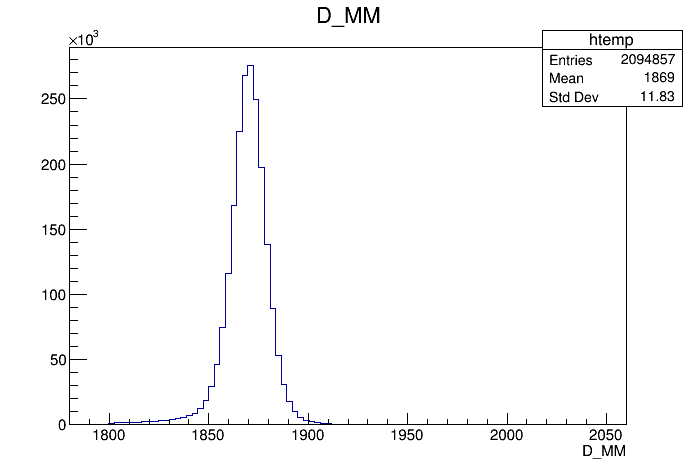
The background sample is composed of events populating the center wing of the invariant mass distribution, between 1910 and 1930 MeV. The sample have 85% magnet Down events and 15 % magnet Up due to the merging between magUp and magDown sample: first the sample was merged and then cut on the first 2094857 events to account for the same number of entries availiable in the MC sample.
The figure below shows the input variables.
The invariant mass of the signal and background is shown below:
The table below shows the configuration of the training:
BDT output
| Correlation matrix | |
|---|---|
| Signal | Background |
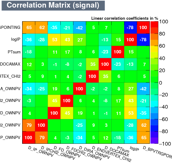 |
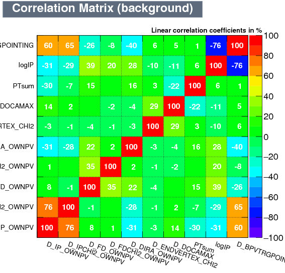 |
| Rejection Background vs Signal efficiency |
|---|
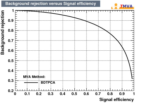 |
| Classifiers | |
|---|---|
| Parameter | BDTPCA |
| Output | 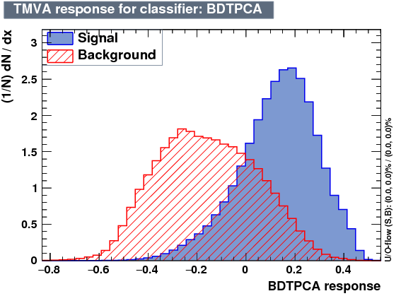 |
| Efficiencies | 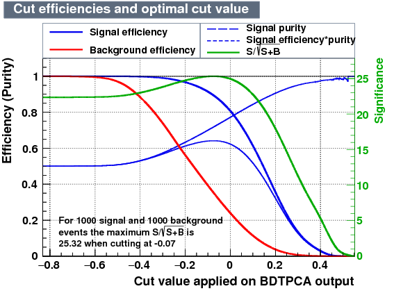 |
| Overtrain | 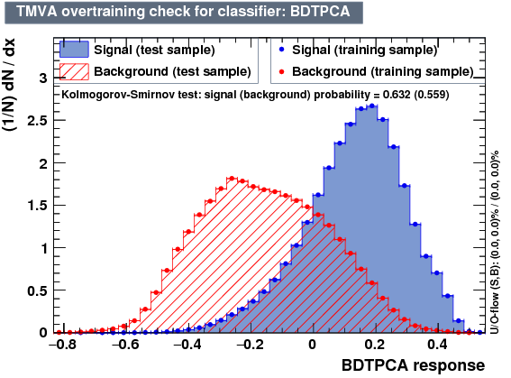 |
Invariant mass spectrum
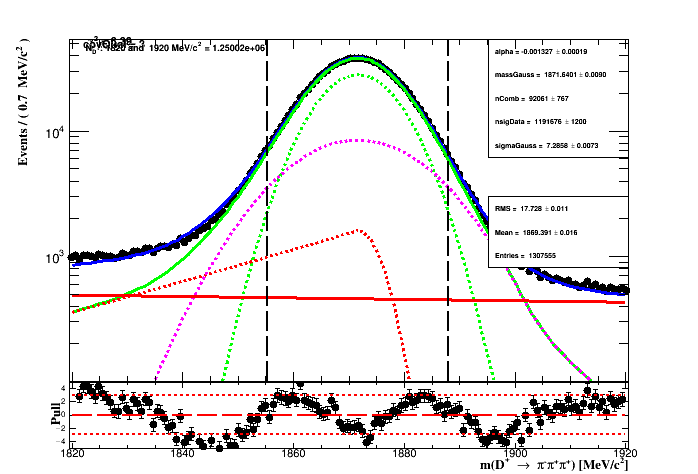
The signal PDF is composed of a Gaussian, taken as the core of the signal model, plus two Crystal-Ball function. Each crystal ball consists of a Gaussian core portion and a power-law low-end tail, below a certain threshold. The function itself and its first derivative are both continuous. Due to the radiative tail of the signal distribution (shown previously here) the crystal ball have different sign of its alpha parameter to allow for better description of the signal tails.
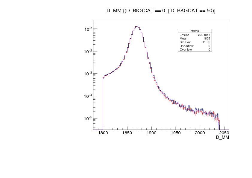
The signal PDF are extracted from the unbinned log-likelihood fit to the D_MM variable of the total 2012 MC sample avaiable consisting of 1M* events. The MC sample is the result of the merging of the old and new (_2017) MC samples with (BKG_CAT == 0 || BKG_CAT == 50). For completeness, the figure below shows the comparioson of the D_MM variable between the old and the new MC sample.
The result of the fit to the MC sample is shown in the figure below.
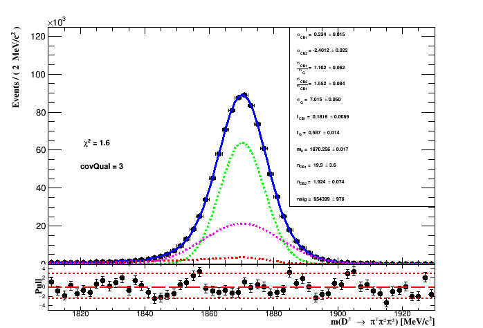
The backgrond contribution is assumed to be combinatorial only and it is described as a expoential. In order to suppress the background in the invariant mass spectrum two cuts are applied:
- p1_PIDK < -1
- BDT > 0.3 .
- alpha_CB1
- alpha_CB2
- n_CB1
- n_CB2
while fixing the ratios R_CB1 and R_CB2 of the signal, means that the proportion of each width of the signal component of the fit to the MC sample is the same on the fit to data. During the fit to data only the yields of the signal and background, the common mass (m_0), the gaussian width and slope of the exponential is left to float. The figure below shows the fit result.
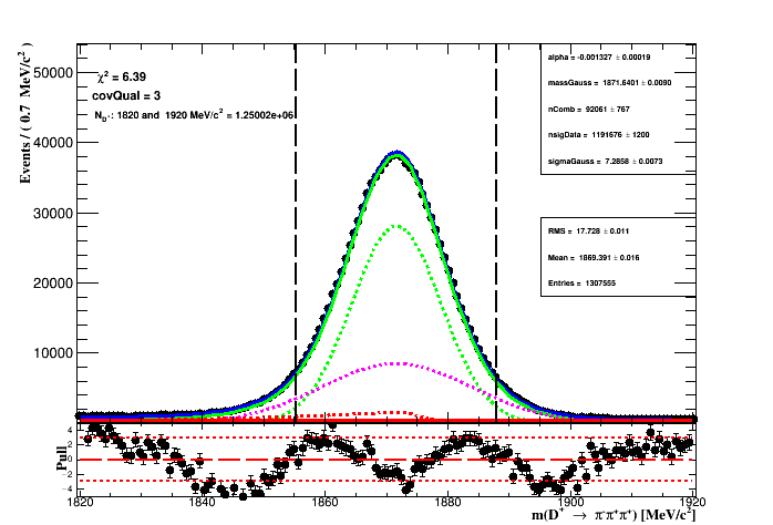
The table below shows the result of the fit with their range. From the fit to data the region of 2*sigma_eff is represented by the vertical lines on the figure of the fit results.
The effective width is of the pdf model is:
 where f_1 and f_G are the fractions of the crystal-ball 1 and the Gaussian respectively.
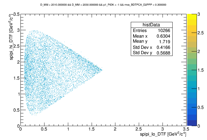
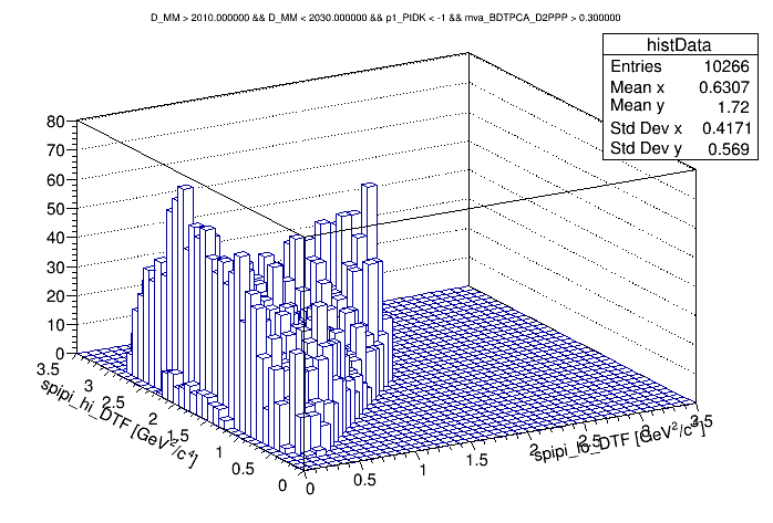
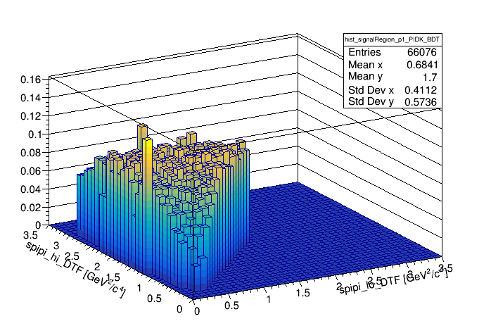
The signal region is: (1855.24 < D_MM < 1888.04) MeV. The number of events in the
2*sigma region is : 109592e+06 while the signal yeild is 106338e+06.
The purity of the selection is the signal yield in the 2*sigma region
(given by the
integral of the PDF* times the
signal yeild*
in the region of the fit) divided by the
number of events in the region.
The expected purity if of 97.0311%*.
where f_1 and f_G are the fractions of the crystal-ball 1 and the Gaussian respectively.
The signal region is: (1855.24 < D_MM < 1888.04) MeV. The number of events in the
2*sigma region is : 109592e+06 while the signal yeild is 106338e+06.
The purity of the selection is the signal yield in the 2*sigma region
(given by the
integral of the PDF* times the
signal yeild*
in the region of the fit) divided by the
number of events in the region.
The expected purity if of 97.0311%*.
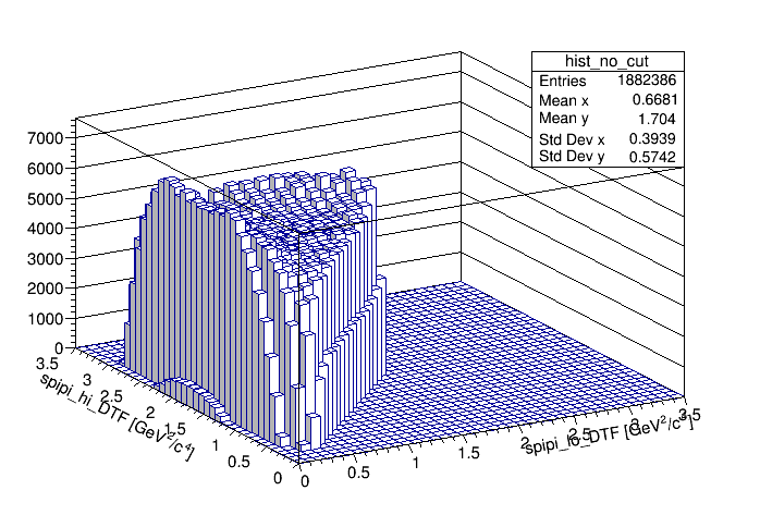
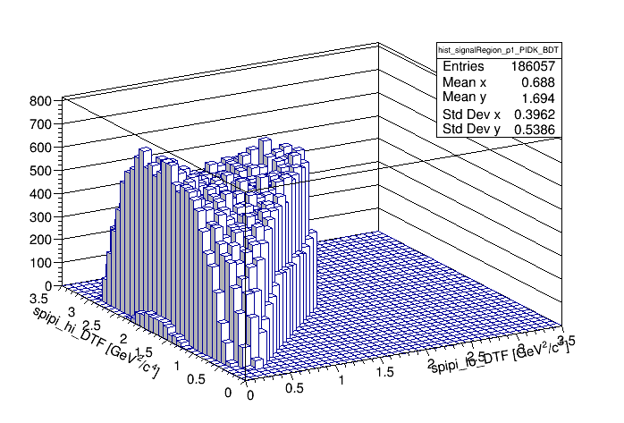
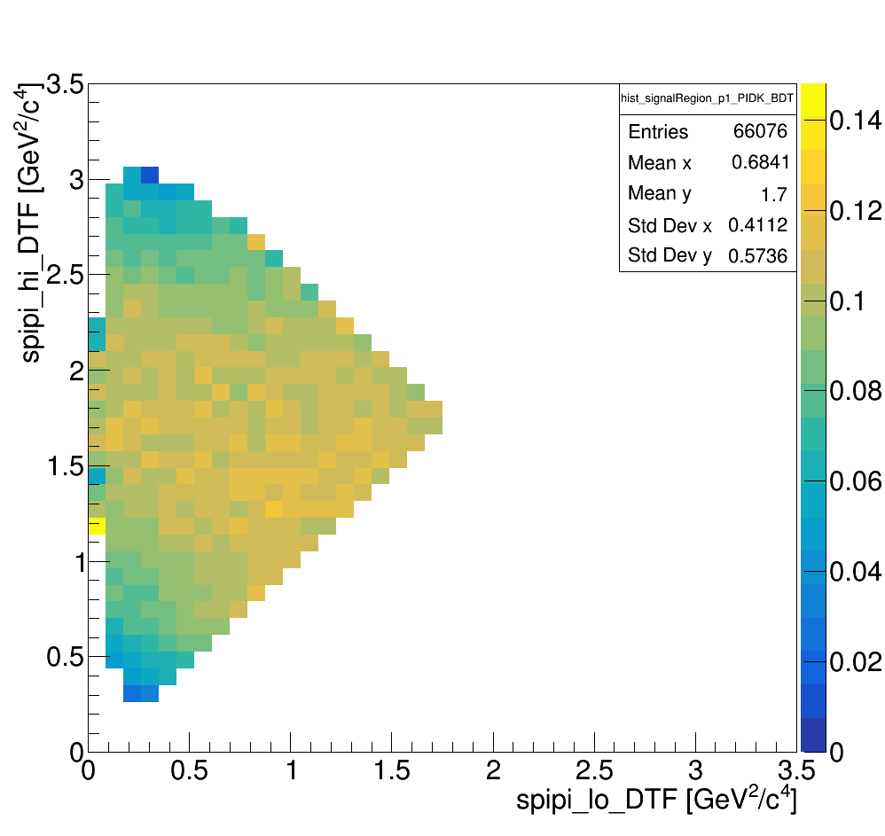
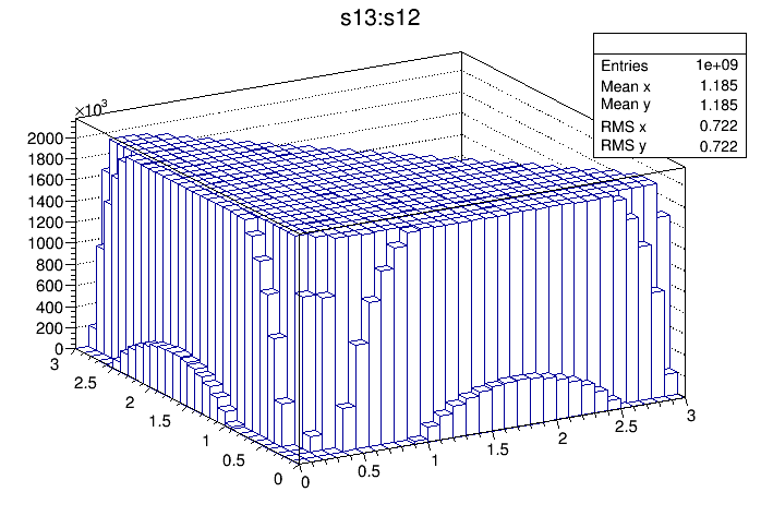
The Dalitz plot of the selection is shown in the figure below:
Dalitz of the bkg regions
Dalitz without any cut
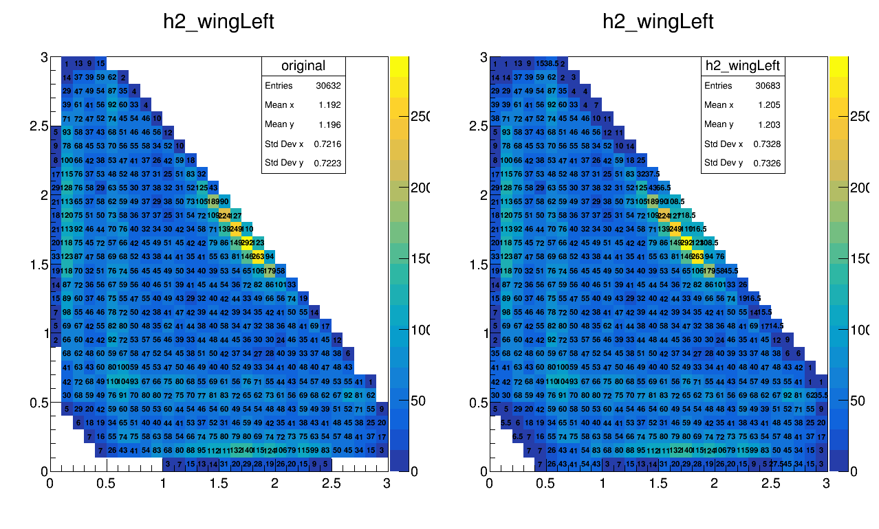
wing left
wing center
wing right
Dalitz with p1_PIDK < -1
wing left
wing center
wing right
Dalitz with p1_PIDK < -1 and BDT > 0.3
wing left
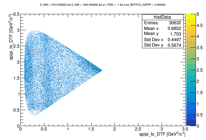
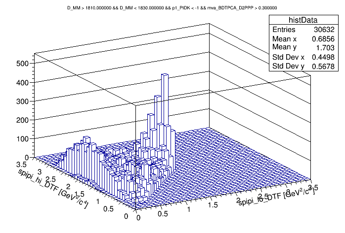
wing center
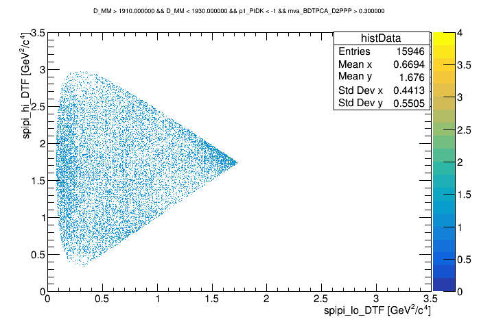
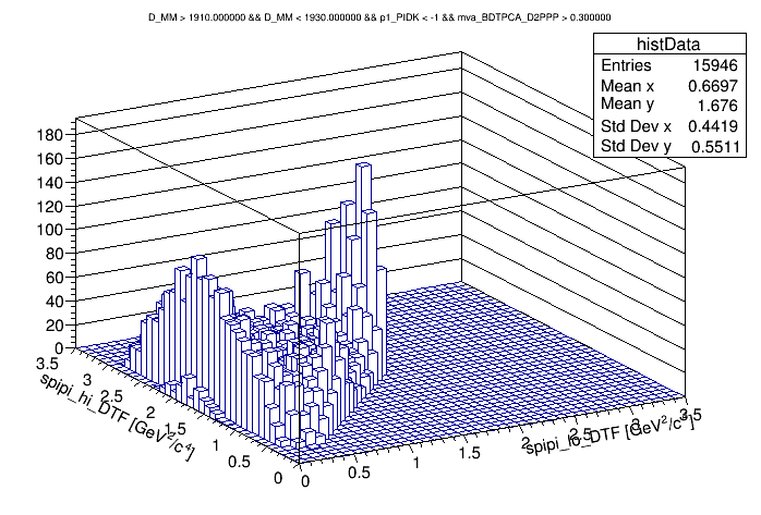
wing right
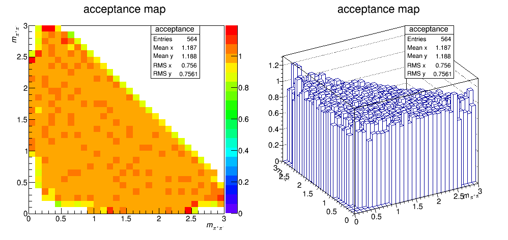
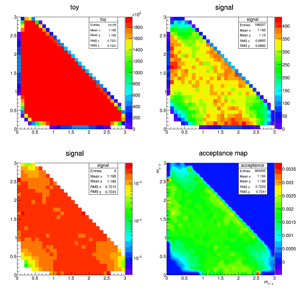
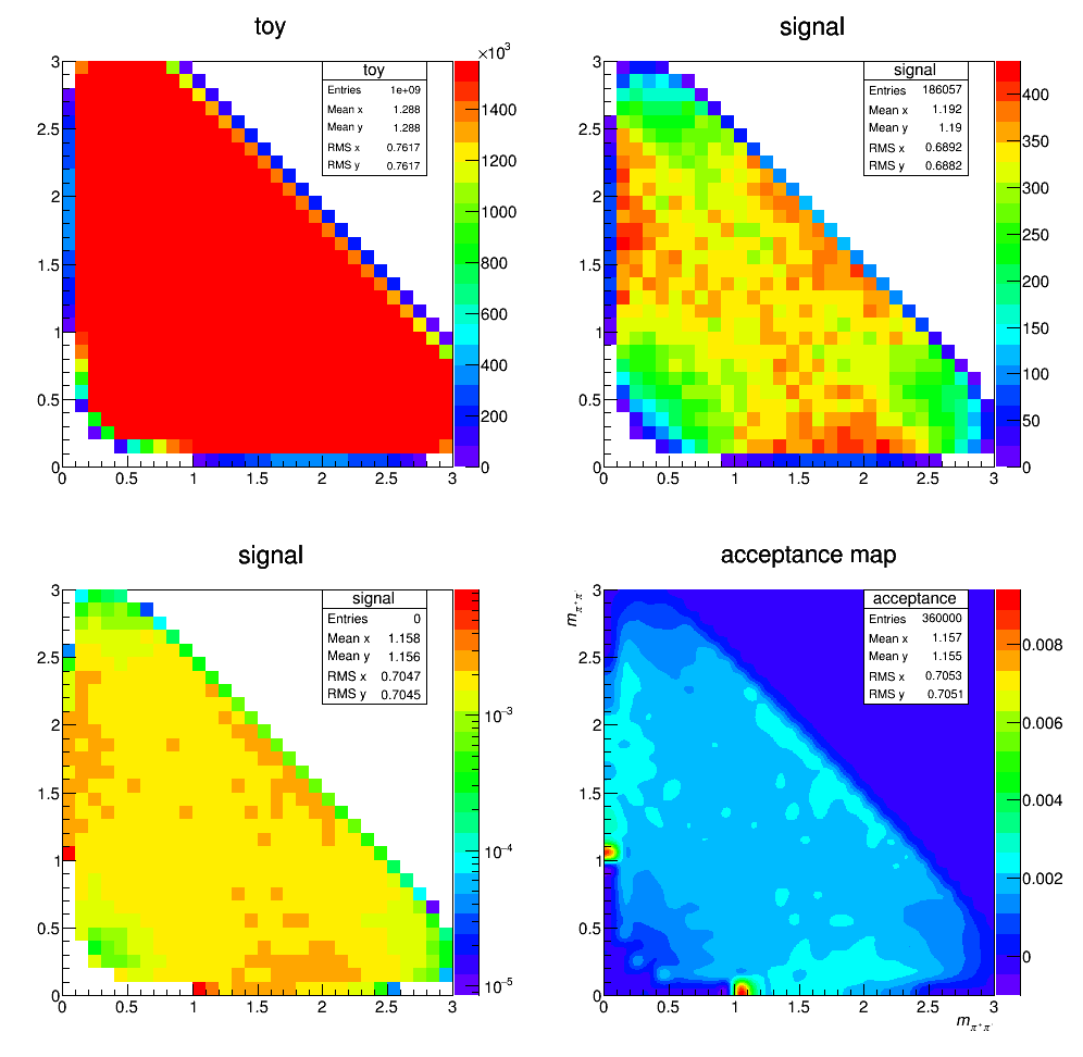
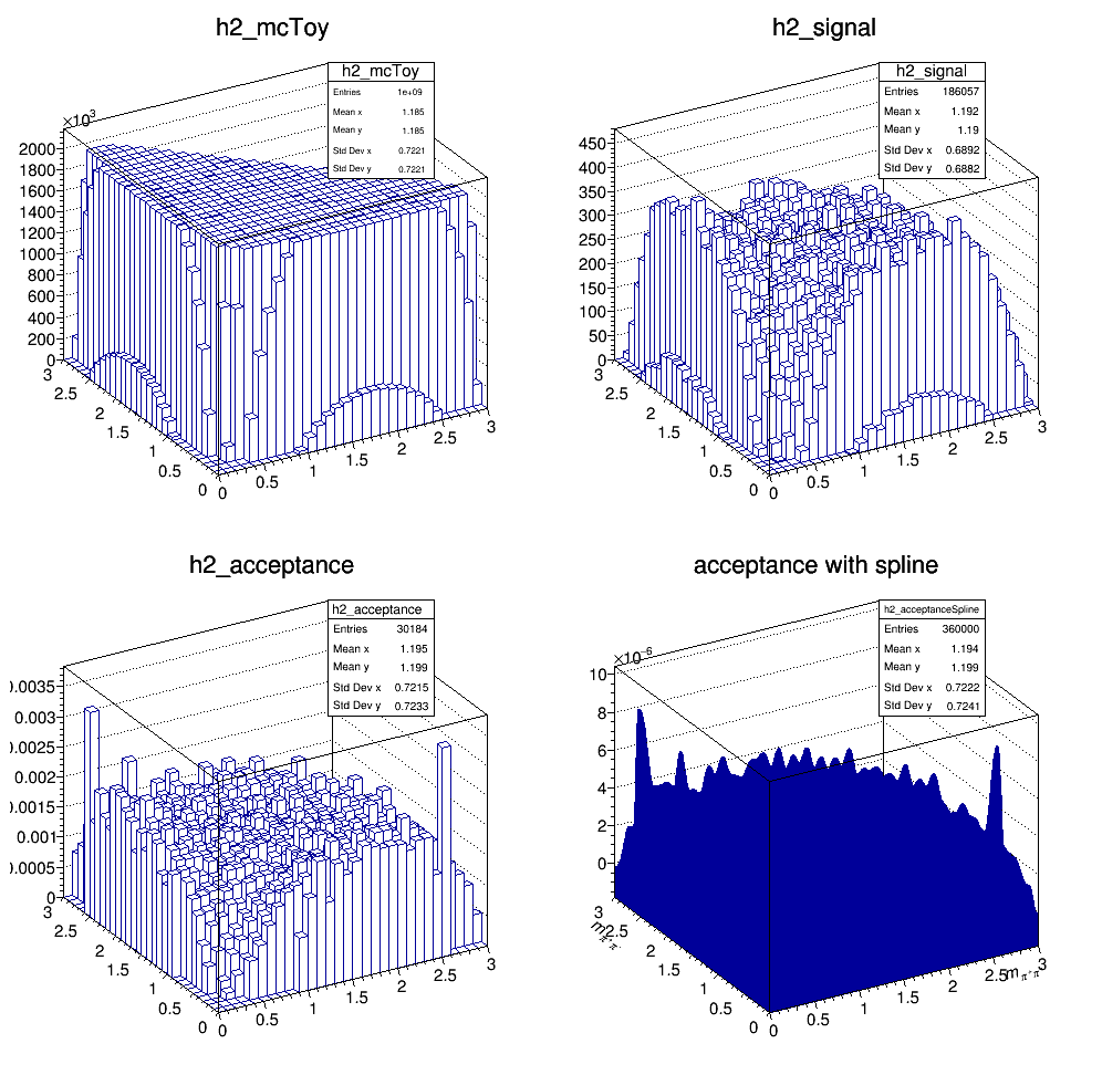
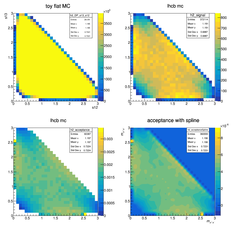
Acceptance
Update 29/09/2017
Selection efficiencies
There are known differences between the L0 simulation and the data. However, the L0 trigger requirement needs to be made in the MC since the our inclusive trigger line StrippingD2hhh_PPPLine, since it has a requirement on the Hlt1TrackAllL0, the L0 trigger requirement needs to be made in the MC. Data-driven methods are applied to account for PID efficiency and to correct for the L0 trigger simulation. The PIDCalib tool is used to determine the PID absolute efficiency, the L0 trigger correction is determined from the efficiency tables, following same procedure of the this analysis.
| Correlation matrix | ||
|---|---|---|
| Cumulative cuts | events | realtive fraction |
| Stripping | 2094857 | 100% |
| 2sigma window | 1882386 | 89.86% |
| PID_p1 | 1700726 | 81.18% |
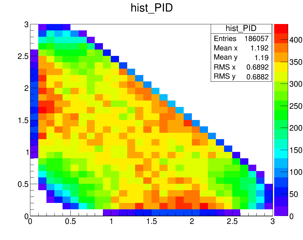
| BDT | 186057 | 8.88% |
| D_L0HadronDecision_TIS | 91690 | 4.38% |
| D_L0HadronDecision_TIS not D_L0HadronDecision_TIS | 69759 | 3.33% |
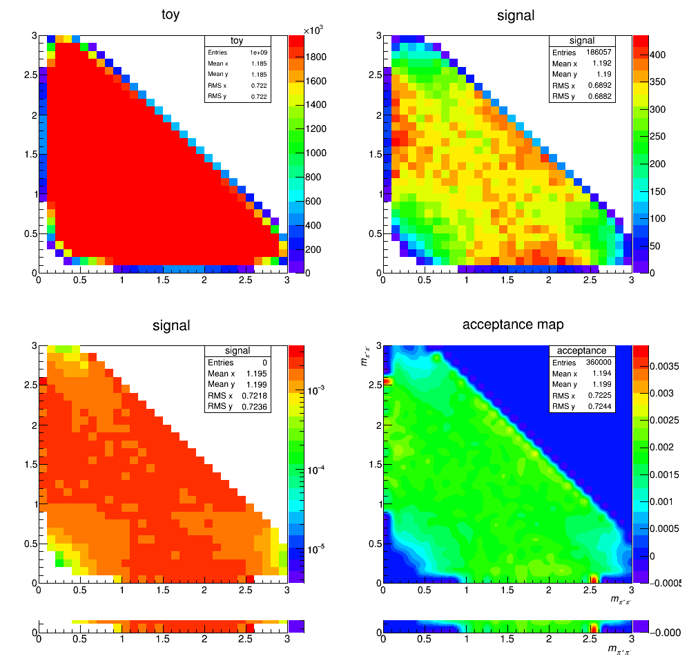
Efficiency histograms including geometrical acceptance, reconstruction and selection efficiency. Neither the effects of PID nor the L0 efficiency correction are considered at this stage. The histograms containing the selected LHCb MC events are divided by a histogram made from a very large ToyMC sample generated with constant matrix element. This division accounts for the bins not entirely contained in the phase space.
Efficiency map (PID and not applied)
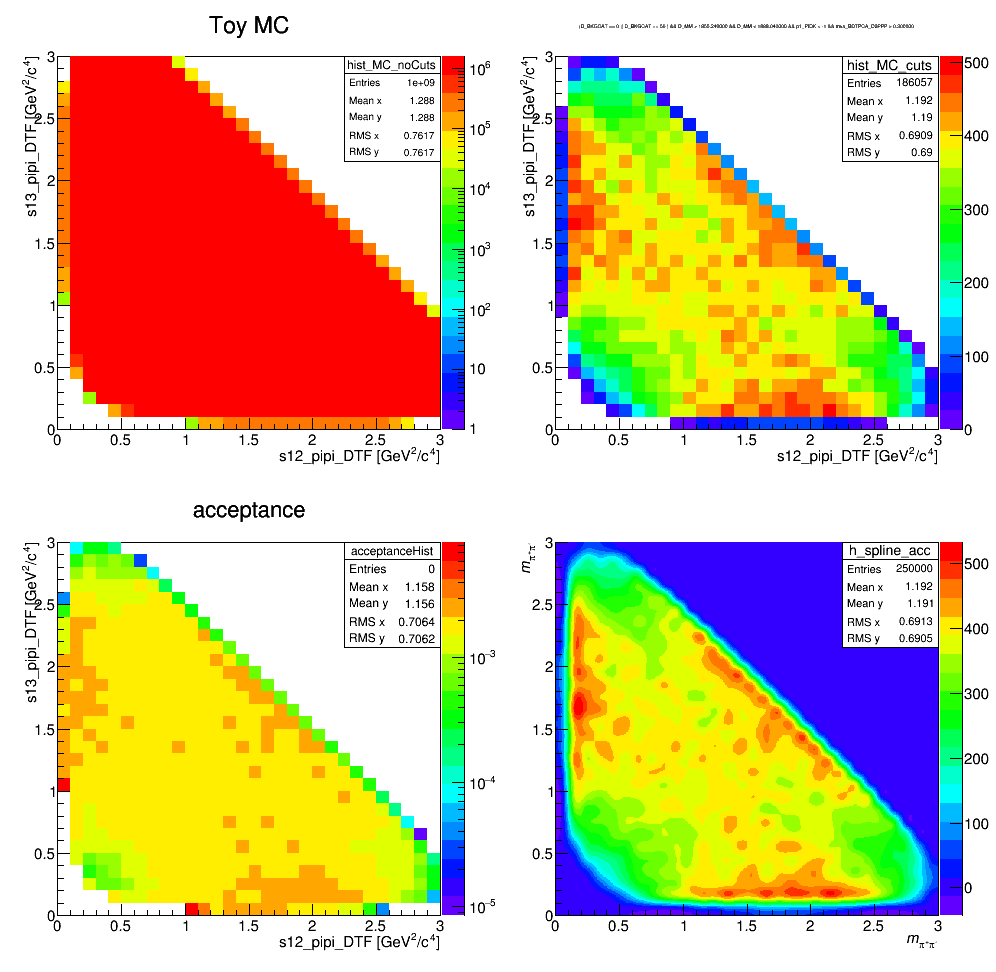
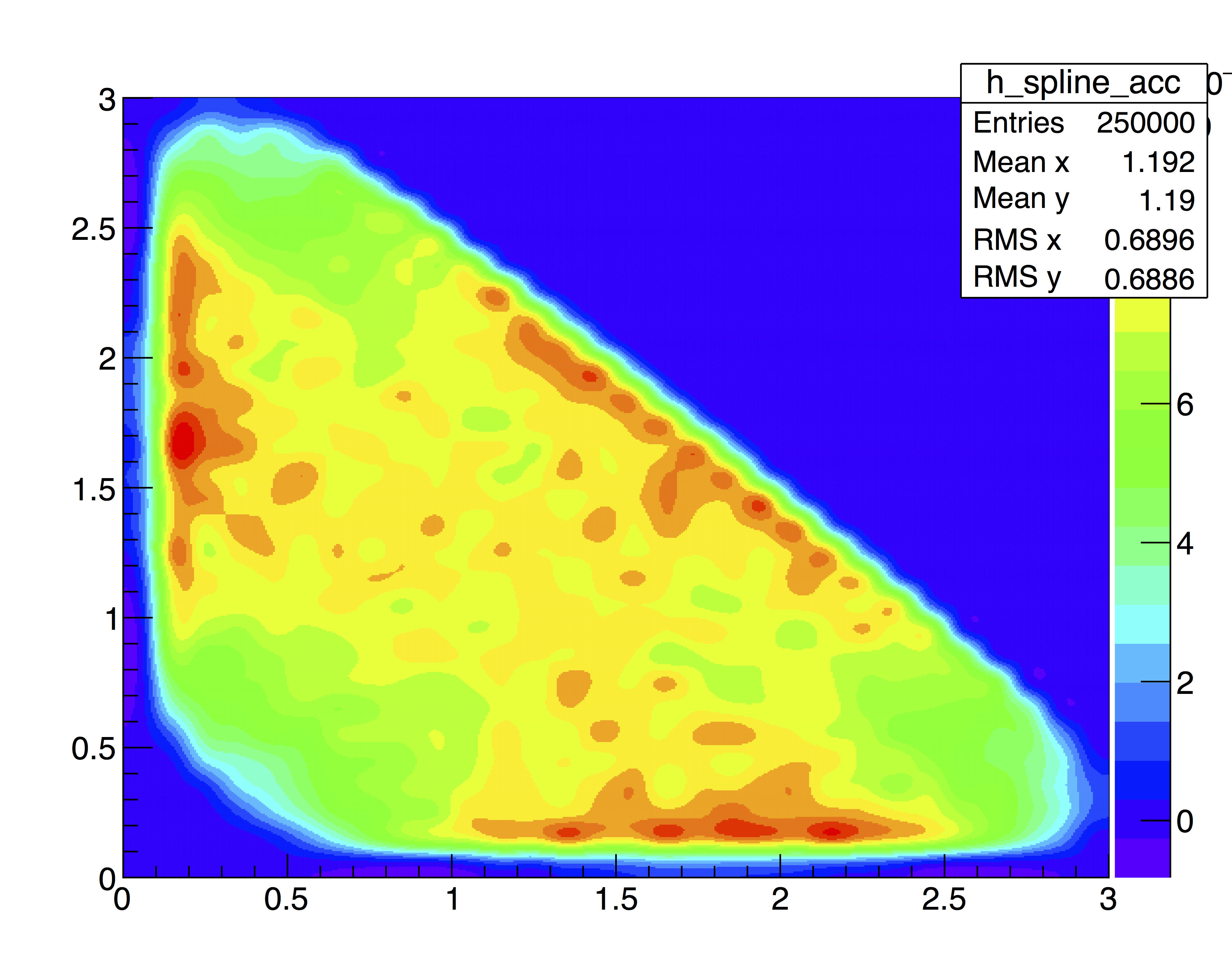
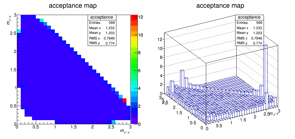
The efficiency distribution is fitted with a two-dimensional cubic spline to smooth out statistical fluctuations due to limited size of the simulated sample. This fit is performed using the Laura++ libraries.
Efficiency map (with PID)
Corretions for TOS
Need to implement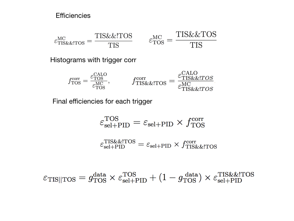
Updates on 02/10/2017
Several changes on the analysis are listed below and are not implemented (yet):
- run again with p1_PIDK < -2
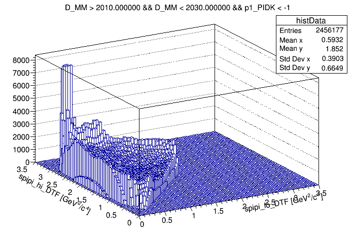
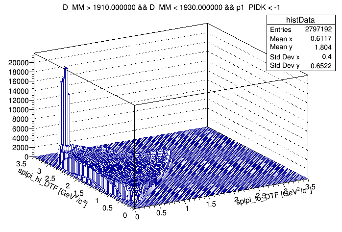
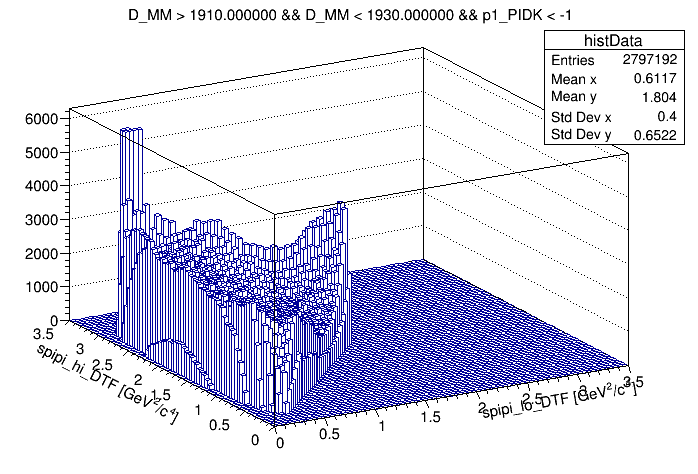
- generate bkg samples with three wings
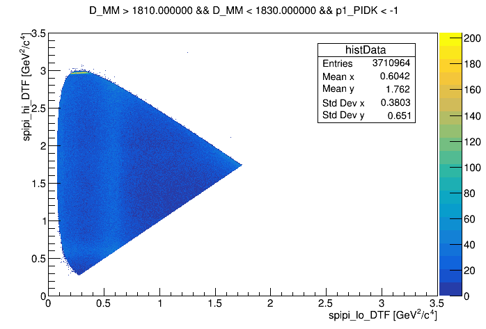
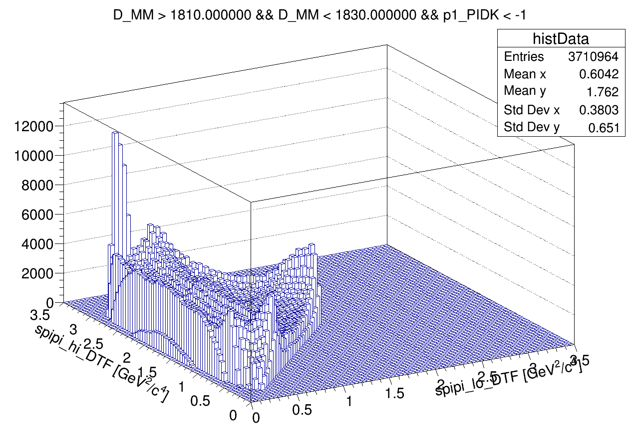
- wing-left: (1810 < D_MM < 1830) MeV
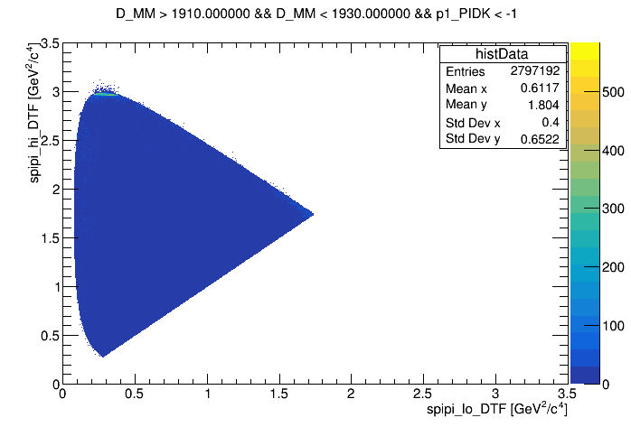
- wing-center: (1910 < D_MM < 1930) MeV
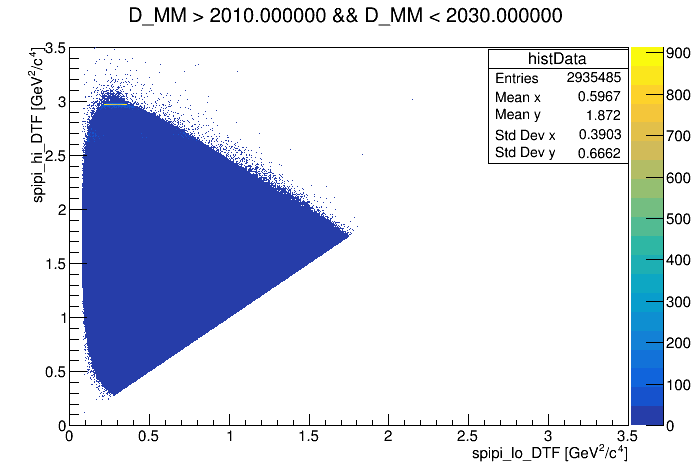
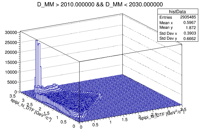
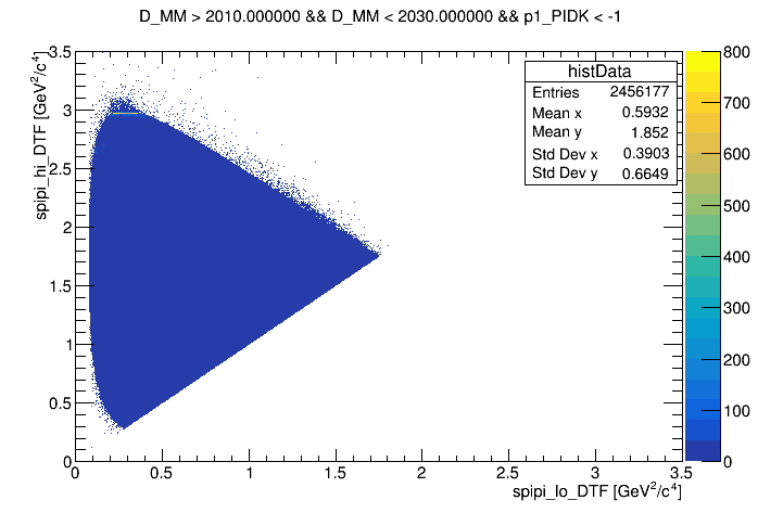
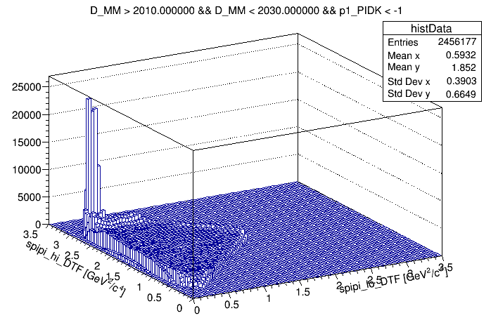
- wing-right: (2010 < D_MM < 2030) MeV
- include isMuon for daughters
Update on 10/10/2017
Acceptance update
- fix mass of the mother
Rio+ fit studies
Performing studies for Rio+ fit. The aim is get proficiency with the Rio+ generating and fitting methods. The list below shows the stemps to be performed.
- Generate a toy MC with defined parameters
- Create a model input to perform the fit
- Verify whether the fitted parameters are close to the defined values during the generation step.
Model for generate toy MC:
Generated sample: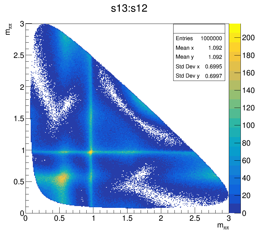
Input of fit
Fit result:Update on 13/10/2017
Acceptance update
We update the mass of the D+ from 1.86959 MeV (from PDG) to 1.86962 MeV (from DTF values). Then rebuild the acceptance map as before. The result is below:

Background
Background from the left (1810, 1830) MeV and right (1910,1930) MeV wings. Dalitz and spline are build as the signal. Result below;
Update on 19/10/2017
Acceptance update
We recalculate the efficiency map across Dalitz plot but using the wrong mass of D. We assume the Ds mass instead of D+ mass in order to reproduce the old result from 29/09/2017 (result before accidently erase my files). The result is below.
A bug was find in the code. The history of the bug fixing is as follow:
- results/19_10_2017_v4 --- bug spoted
- results/19_10_2017_v5 --- bug fix test
- results/19_10_2017_v6 --- bug fix implemented
   56   //Creating the histograms;
   57
   58   TH2F * h2mcLHCbSignal = MakeHistogram("signal",nbins,mcLHCbFile);
   59   TH2F * h2mcToy        = MakeHistogram("toy"   ,nbins,mcToyFile);
   60
   61   //TH2F *h2Acceptance = (TH2F*)h2mcLHCbSignal->Clone("h2Acceptance");
   62   TH2F *h2Acceptance = MakeHistogram("signal",nbins,mcLHCbFile);
   63
   64   h2Acceptance->Divide(h2mcToy);
Which change by
   55   //Creating the histograms;
   56   TH2F * h2_signal     = MakeHistogram("h2_signal",nbins,mcLHCbFile);
   57   TH2F * h2_mcToy      = MakeHistogram("h2_mcToy"   ,nbins,mcToyFile);
   58   TH2F * h2_acceptance = MakeHistogram("h2_acceptance",nbins,mcLHCbFile);
   59
   60   h2_acceptance->Divide(h2_mcToy);
with changes appropriate names below those lines.
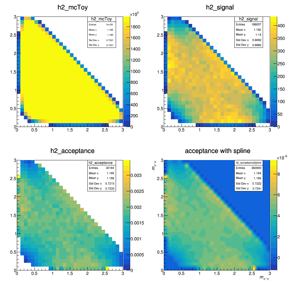
The current acceptance map is then:
Update on 25/10/2017
Toy MC
Bkg 1810 - 1830 MeV DP
Bkg 1910 - 1930 MeV DP
Acceptance 1810 - 1830 MeV DP
Acceptance 1910 - 1930 MeV DP
Spline Acceptance 1810 - 1830 MeV DP
Spline Acceptance 1910 - 1930 MeV DP
Ratio: rebined spline / acceptance (bkg: 1810 - 1830) MeV
Ratio: rebined spline / acceptance (bkg: 1910 - 1930) MeV
Update on 26/10/2017
Bkg 1810 - 1830 MeV DP (with extra binning)
Example of the extra-binning method on the bkg (1810,1830) MeV
Update on 27/10/2017
Update on the acceptance
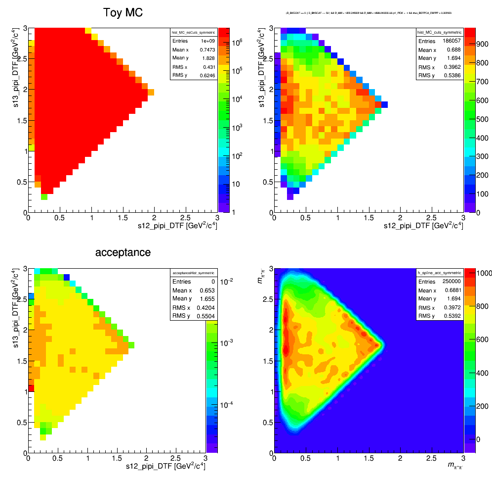
Update includes the extra binning on the efficiency map of the simetrical signal and background DP
LHCb MC signal
LHCb MC acceptance (signal / toy mc)
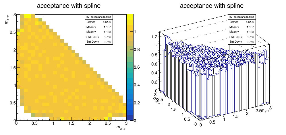
LHCb MC acceptance spline fit
spline fit rebin / acceptance
Signal acceptance with extra bins
Signal acceptance spline fit with extra bins
spline fit rebin with extra bin / acceptance
acceptance with extra bin - acceptance
Background
DP: wing 1810 - 1830
DP: wing 1910 - 1930
DP: LHCb MC / toy MC wing 1810 - 1830
DP: LHCb MC / toy MC wing 1910 - 1930
DP: spline fit wing 1810 - 1830
DP: spline fit wing 1910 - 1930
DP: Ratio spline / acceptance 1810 - 1830
DP: Ratio spline / acceptance 1910 - 1930
DP: accep with extra bin 1810 - 1830
DP: accep with extra bin 1910 - 1930
DP: spline fit with extra bin 1810 - 1830
DP: spline fit with extra bin 1910 - 1930
DP: spline fit with extra bin 1810 - 1830
DP: spline fit with extra bin 1910 - 1930
DP: (acceptance with extra bin rebined - acceptance) 1810 - 1830
DP: (acceptance with extra bin rebined - acceptance) 1910 - 1930
Update on 30/10/2017
Rio+ fit studies:
Test 1: FCN = 149552.41
| MC Generation and Fit | ||||||
|---|---|---|---|---|---|---|
| Ressonance | Generate with | Start fit with | Fit result | |||
| Re | Im | Re | Im | Re | Im | |
| rho(770) pi | 1.0 | 0 | 1.0 | 0 | 1.0 | 0 |
| rho(1450) pi | 0.6 | -0.3 | 0.8 | -0.2 | 0.603±0.003 | -0.291 ±0.006 |
| f21270+pi | 0.7 | -0.5 | 0.2 | -0.3 | 0.712±0.009 | -0.498 ±0.009 |
| f21525+pi | 0.3 | -0.4 | 0.5 | -0.1 | 0.285±0.026 | -0.407 ±0.031 |
Test 2: (with NR) FCN = 148360.967
| MC Generation and Fit | ||||||
|---|---|---|---|---|---|---|
| Ressonance | Generate with | Start fit with | Fit result | |||
| Re | Im | Re | Im | Re | Im | |
| 3pi_NR | 0.5 | -0.5 | 0.2 | -0.1 | 0.2±74.778 | -0.100±74.652 |
| rho(770) pi | 1.0 | 0 | 1.0 | 0 | 1.0 | 0 |
| rho(1450) pi | 0.6 | -0.3 | 0.8 | -0.2 | 0.597±0.004 | -0.284 ±0.006 |
| f21270+pi | 0.7 | -0.5 | 0.2 | -0.3 | 0.687±0.009 | -0.512 ±0.009 |
| f21525+pi | 0.3 | -0.4 | 0.5 | -0.1 | 0.321±0.026 | -0.319 ±0.032 |
However I found later that:
                         42  PARAMETER DEFINITIONS:
                         43     NO.   NAME         VALUE      STEP SIZE      LIMITS
                         44      1 3pi_NR_re    2.00000e-01  1.00000e-05   -5.00000e+01  5.00000e+01
                         45      2 3pi_NR_im   -1.00000e-01  1.00000e-05   -5.00000e+01  5.00000e+01
                         46      3 3pi_NR_mass   0.00000e+00  1.00000e-05    0.00000e+00  1.00000e+00
                         47  MINUIT WARNING IN PARAM DEF
                         48  ============== STARTING VALUE IS AT LIMIT.
                         49  MINUIT WARNING IN PARAMETR
                         50  ============== VARIABLE3 IS AT ITS LOWER ALLOWED LIMIT.
                         51  MINUIT WARNING IN PARAMETR
                         52  ============== VARIABLE3 BROUGHT BACK INSIDE LIMITS.
                         53      4 3pi_NR_width   0.00000e+00  1.00000e-05    0.00000e+00  1.00000e+00
                         54  MINUIT WARNING IN PARAM DEF
                         55  ============== STARTING VALUE IS AT LIMIT.
                         56  MINUIT WARNING IN PARAMETR
                         57  ============== VARIABLE4 IS AT ITS LOWER ALLOWED LIMIT.
                         58  MINUIT WARNING IN PARAMETR
                         59  ============== VARIABLE4 BROUGHT BACK INSIDE LIMITS.
                         60      5 3pi_NR_res_extra_par_0   0.00000e+00  1.00000e-05   -2.00000e+01  2.00000e+01
                         61      6 3pi_NR_res_extra_par_1   0.00000e+00  1.00000e-05   -2.00000e+01  2.00000e+01
                         62      7 3pi_NR_res_extra_par_2   0.00000e+00  1.00000e-05   -2.00000e+01  2.00000e+01
                         63      8 3pi_NR_res_extra_par_3   0.00000e+00  1.00000e-05   -2.00000e+01  2.00000e+01
Update on 31/10/2017
After fix the warning, due to the mass and the width of the NR3pi are set to the lower limit of the parameter the problem still persists:
Test 3: (with NR) FCN = 148360.932
| MC Generation and Fit | ||||||
|---|---|---|---|---|---|---|
| Ressonance | Generate with | Start fit with | Fit result | |||
| Re | Im | Re | Im | Re | Im | |
| 3pi_NR | 0.5 | -0.5 | 0.2 | -0.1 | -23.620±59.650 | -0.6±74.439 |
| rho(770) pi | 1.0 | 0 | 1.0 | 0 | 1.0 | 0 |
| rho(1450) pi | 0.6 | -0.3 | 0.8 | -0.2 | 0.597±0.003 | -0.284 ±0.006 |
| f21270+pi | 0.7 | -0.5 | 0.2 | -0.3 | 0.687±0.009 | -0.512 ±0.005 |
| f21525+pi | 0.3 | -0.4 | 0.5 | -0.1 | 0.321±0.022 | -0.319 ±0.026 |
Test 4: (with NR and f0(980)) FCN = 194082.197
| MC Generation and Fit | ||||||
|---|---|---|---|---|---|---|
| Ressonance | Generate with | Start fit with | Fit result | |||
| Re | Im | Re | Im | Re | Im | |
| f0(980) | 0.9 | -0.2 | 0.6 | -0.1 | -0.003±0.000 | -0.005±0.000 |
| 3pi_NR | 0.5 | -0.5 | 0.2 | -0.1 | 0.238±74.794 | -0.102±74.651 |
| rho(770) pi | 1.0 | 0 | 1.0 | 0 | 1.0 | 0 |
| rho(1450) pi | 0.6 | -0.3 | 0.8 | -0.2 | 0.514±0.005 | -0.077 ±0.005 |
| f21270+pi | 0.7 | -0.5 | 0.2 | -0.3 | 0.765±0.010 | -0.560 ±0.009 |
| f21525+pi | 0.3 | -0.4 | 0.5 | -0.1 | 0.770±0.030 | -0.660 ±0.029 |
Test 5: (with omega) FCN = 130724.872
| MC Generation and Fit | ||||||
|---|---|---|---|---|---|---|
| Ressonance | Generate with | Start fit with | Fit result | |||
| Re | Im | Re | Im | Re | Im | |
| omega pi | 0.9 | -0.3 | 0.6 | -0.5 | 0.957±0.013 | -0.130±0.016 |
| rho(770) pi | 1.0 | 0 | 1.0 | 0 | 1.0 | 0 |
| rho(1450) pi | 0.6 | -0.3 | 0.8 | -0.2 | 0.602±0.004 | -0.285 ±0.006 |
| f21270+pi | 0.7 | -0.5 | 0.2 | -0.3 | 0.726±0.010 | -0.467 ±0.011 |
| f21525+pi | 0.3 | -0.4 | 0.5 | -0.1 | 0.357±0.028 | -0.437 ±0.031 |
Test 6: (with f0X(m0 = 1.430, w0 = 0.180 )) FCN = 217274.068
| MC Generation and Fit | ||||||
|---|---|---|---|---|---|---|
| Ressonance | Generate with | Start fit with | Fit result | |||
| Re | Im | Re | Im | Re | Im | |
| f0(X) pi | 0.5 | -0.4 | 0.3 | -0.5 | 0.502±0.004 | -0.400±0.007 |
| rho(770) pi | 1.0 | 0 | 1.0 | 0 | 1.0 | 0 |
| rho(1450) pi | 0.6 | -0.3 | 0.8 | -0.2 | 0.597±0.008 | -0.303 ±0.011 |
| f21270+pi | 0.7 | -0.5 | 0.2 | -0.3 | 0.715±0.013 | -0.495 ±0.011 |
| f21525+pi | 0.3 | -0.4 | 0.5 | -0.1 | 0.308±0.036 | -0.331 ±0.052 |
Test 7: (with f0(1500)) FCN = 210188.314
| MC Generation and Fit | ||||||
|---|---|---|---|---|---|---|
| Ressonance | Generate with | Start fit with | Fit result | |||
| Re | Im | Re | Im | Re | Im | |
| f0(1500) pi | 0.8 | -0.6 | 0.6 | -0.3 | 0.796±0.006 | -0.602±0.010 |
| rho(770) pi | 1.0 | 0 | 1.0 | 0 | 1.0 | 0 |
| rho(1450) pi | 0.6 | -0.3 | 0.8 | -0.2 | 0.608±0.010 | -0.294 ±0.010 |
| f21270+pi | 0.7 | -0.5 | 0.2 | -0.3 | 0.705±0.011 | -0.479 ±0.011 |
| f21525+pi | 0.3 | -0.4 | 0.5 | -0.1 | 0.391±0.044 | -0.551 ±0.077 |
Test 8: (with f0(1710) ) FCN = 163371.982
| MC Generation and Fit | ||||||
|---|---|---|---|---|---|---|
| Ressonance | Generate with | Start fit with | Fit result | |||
| Re | Im | Re | Im | Re | Im | |
| f0(1710) pi | 0.5 | -0.4 | 0.3 | -0.7 | 0.501±0.005 | -0.403±0.004 |
| rho(770) pi | 1.0 | 0 | 1.0 | 0 | 1.000 | 0.000 |
| rho(1450) pi | 0.6 | -0.3 | 0.8 | -0.2 | 0.603±0.005 | -0.287±0.007 |
| f21270+pi | 0.7 | -0.5 | 0.2 | -0.3 | 0.721±0.009 | -0.489±0.009 |
| f21525+pi | 0.3 | -0.4 | 0.5 | -0.1 | 0.290±0.032 | -0.559±0.034 |
Test 9: (with f0(980) ) FCN = 198081.120
| MC Generation and Fit | ||||||
|---|---|---|---|---|---|---|
| Ressonance | Generate with | Start fit with | Fit result | |||
| Re | Im | Re | Im | Re | Im | |
| f0(1710) pi | 0.5 | -0.4 | 0.3 | -0.7 | -0.002±0.000 | -0.005±0.000 |
| rho(770) pi | 1.0 | 0 | 1.0 | 0 | 1.000 | 0.000 |
| rho(1450) pi | 0.6 | -0.3 | 0.8 | -0.2 | 0.516 ±0.005 | -0.078±0.005 |
| f21270+pi | 0.7 | -0.5 | 0.2 | -0.3 | 0.779 ±0.007 | -0.584±0.008 |
| f21525+pi | 0.3 | -0.4 | 0.5 | -0.1 | 0.788 ±0.029 | -0.881±0.030 |
Test 10: (test amplitude and phase ): FCN = 252962.716
| MC Generation and Fit | ||||||
|---|---|---|---|---|---|---|
| Ressonance | Generate with | Start fit with | Fit result | |||
| Amp | Phs | Amp | Phs | Amp | Phs | |
| f0(1500) pi | 0.2 | 45 | 0.4 | 40 | 0.204 ±0.006 | 43.380 ±1.466 |
| f0(1710) pi | 0.9 | 90 | 0.5 | 80 | 0.893 ±0.006 | 90.113 ±0.814 |
| rho(770) pi | 1 | 0 | 1 | 0 | 1.000 | 0 |
| rho(1450)+pi | 0.8 | 135 | 0.9 | 110 | 0.807 ±0.007 | 133.561±1.222 |
Test 11: (test amplitude and phase with NR ): FCN = 253908.498
| MC Generation and Fit | ||||||
|---|---|---|---|---|---|---|
| Ressonance | Generate with | Start fit with | Fit result | |||
| Amp | Phs | Amp | Phs | Amp | Phs | |
| 3pi NR | 0.5 | 30 | 0.7 | 20 | 2.709±73.169 | 21.458 ±277.321 |
| f0(1500) pi | 0.2 | 45 | 0.4 | 40 | 0.196±0.005 | 45.965 ±1.028 |
| f0(1710) pi | 0.9 | 90 | 0.5 | 80 | 0.892±0.006 | 90.030 ±0.370 |
| rho(770) pi | 1 | 0 | 1 | 0 | 1.000 0 | 0 |
| rho(1450)+pi | 0.8 | 135 | 0.9 | 110 | 0.799±0.007 | 135.786±0.549 |
Update on 01/11/2017
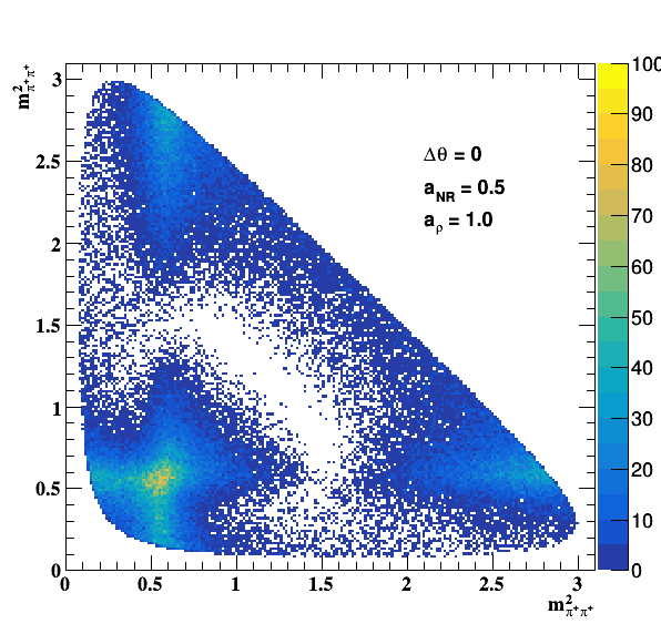
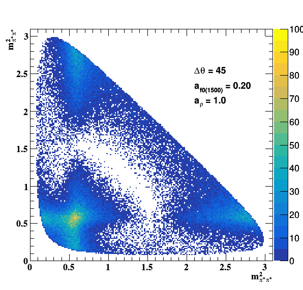
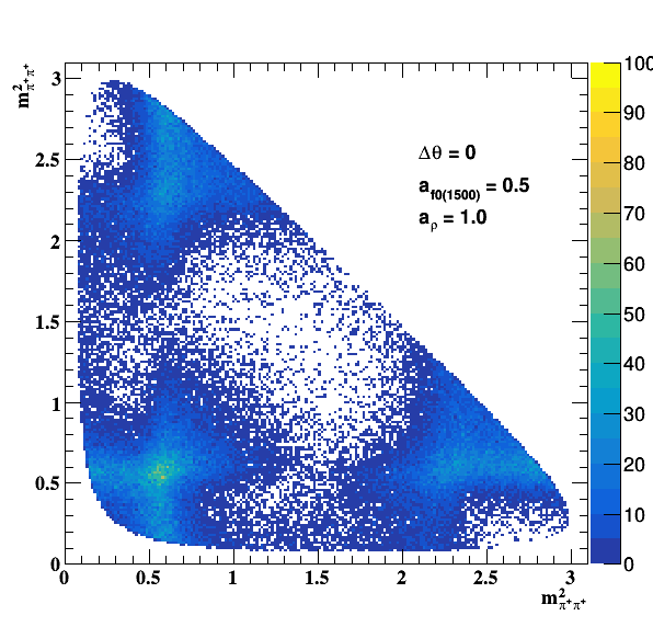
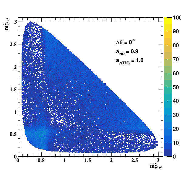
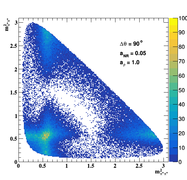
Test of interference NR + ρ(770)
Update on 03/11/2017
Test of interference NR + ρ(770)
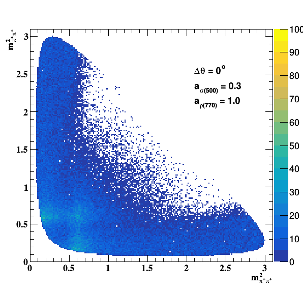
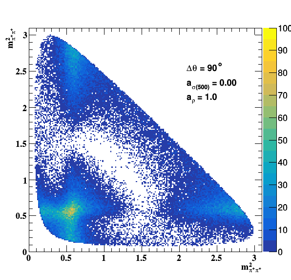
Testing NR and ρ(770) amplitude and fase shift:
Testing ρ(770) and f0(1500) amplitude and fase shift:
Update on 09/11/2017
Fixing bug on NR component of Rio+
File: cernbox/Rio+/Rio+/src/Amplitudes.h lines
                      136         //sig.at(size_resonances) = (1.,0.);
                      137         sig.at(size_resonances) = sig.at(size_resonances).One();
And the NR component is generated as expected
Change in the file shared.h to int GLOBAL_TOY = 1; the fit of f0(980) is do the job... Comparisons with previous table below:
Test 12: (fit with most ressonances, but sigma and S wave NR) FCN = 230475.037| MC Generation and Fit | ||||||
|---|---|---|---|---|---|---|
| Ressonance | Generate with | Start fit with | Fit result | |||
| Amp | Phs | Amp | Phs | Amp | Phs | |
| 3pi_NR | 0.3 | 30 | 0.2 | 40 | 0.288±0.012 | 37.501 ±3.422 |
| f0(980) | 0.5 | 40 | 0.2 | 30 | 0.510±0.024 | 39.312 ±2.443 |
| f0(X) pi | 0.7 | 45 | 0.5 | 30 | 0.725±0.022 | 45.348 ±1.294 |
| f0(1500) pi | 0.45 | 65 | 0.5 | 50 | 0.455±0.015 | 64.695 ±2.261 |
| f0(1710) pi | 0.7 | 90 | 0.4 | 80 | 0.730±0.022 | 93.762 ±2.551 |
| rho(770) pi | 1.0 | 0 | 1.0 | 0 | 1.000±0.000 | 0.000 ±0.000 |
| rho(1450) pi | 0.4 | 160 | 0.8 | 100 | 0.309±0.056 | 163.030±2.696 |
| f21270+pi | 0.6 | 70 | 0.5 | 60 | 0.600±0.016 | 69.785 ±2.298 |
| f21525+pi | 0.8 | 10 | 0.6 | 5 | 0.877±0.087 | 12.571 ±3.620 |
| omega pi | 0.75 | 85 | 0.6 | 75 | 0.900±0.023 | 92.165 ±1.698 |
Update on 14/11/2017
Implement σ(500) with Pole amplitude
Update on 29/11/2017
Updating after change the server
During the breakdown of positron machine several studies on the Rio+ fit were performed. These includes the sanity check of the Rio fit. The idea is to chose a simplified model (isobar), only signal (excluding any background and acceptance effect). Once the model is stablished we generate 1k independent samples and fit each of them to restore the values of the generated values. By this method we expect that the deviation of the amplitude and phase of each ressonances be Gaussian distributed as are the FCN values.
The FCN value should be centered in a single Gaussian distribution. If others values are displaced from the Gaussian (outliers) is seen it means that other local minimum value is found by the fit. Chosing initial values of the fit closer to the generated values should remove such outliers.
Click here to open the slides of the fit result without acceptance and background.
Update on 30/11/2017
Adding background and acceptance to GenFit
Test of the background and acceptance in the Rio+/toy generator. Both tests show that Rio+ successfully can integrate the efficiency map of the signal the background taken from the wings.
The input of the efficiency map for the background to the generator is DP of the LHCb data of the wing (1810 - 1830) smoothen with the spline method. The background is generated with a arbitrary model but with background fraction 1.0. 250k evnts were generate. DP below are symmetrical, then nentries are 500k. Results below:
In order to test whether Rio+ correcly integrate the efficiency map of the signal, we generate a model with 5% of background from eff. map with and without the efficiency from signal. Both models (with and without acceptance) are divided by the large toy mc (1bi evts) and then compared to the efficiency map which is the input of the Rio+. Result below:
Update on 06/12/2017
Test of background and fit
An issue from previous update is the background composition which should be removed by subtracting DP with and without background. To avoid this extra complication we test generate the the flat distribution (NR) with the acceptance taken from previous studies. Result below:
From the ratio between the (NR + acceptance) over the acceptance map of the signal, one can conclude Rio+= succesfully integrates the acceptance map to generate. Next steps towards the fit procedure the is run myGenerator program to check if the result of the fit with 5% bkg and acceptance can reproduce the values of the model used for ntuple generation.