Amplitude Analyses of D →πππ
Prelude: LHCbANA
This web resume the ultimate status of D →πππ analyses.
Selection
TMVA
Three BDT discriminators are the used to train 3815245 simulated events from LHCb (signal) where 1907622 were used for train and 1907622 used to test and evalute the MVA efficiency. The MC configuration are XXXXX.YYYYY sim08. merged with XXXX.YYYYY Sim08 2017 condition. Four weights were applied to this signal ntuple:
- Ntracks weight (diff between number of tracks on data and simulation);
- s_weight (from s-plot method from Root toolkit to enhance the signal);
- PIDeff (efficiency from the PID cut given by the LHCb PIDCalib);
- weight (MVA approach to re-weight the MC variable used to train to data);
The MC sample is made with BKG_CAT == 0 || BKG_CAT == 50 for the signal selection (171530 BKGCAT==50 and 3643715 BKGCAT==0). Those selection also have the magnet UP (1916080 sim. events) and magnet down (1899165 sim. events).
The background sample is composed of events populating the left and right wing of the signal region. The wing from the left (1810 < D_MM < 1830) have 760838 events. The wing at the right of the signal peak (1910 < D_MM < 1930) have 552305 events totalizing 1313143 events where half were used to train and the other half used to evaluate the BDT efficiency. The background selection for training sample have ~ 49 % magnet down events and ~ 51 magnet up.
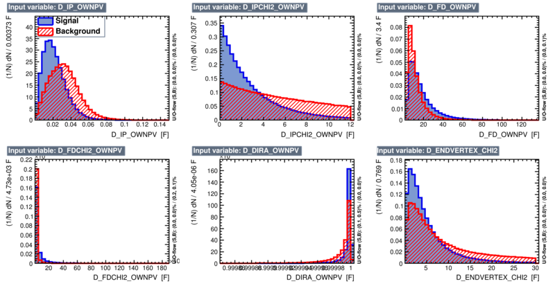
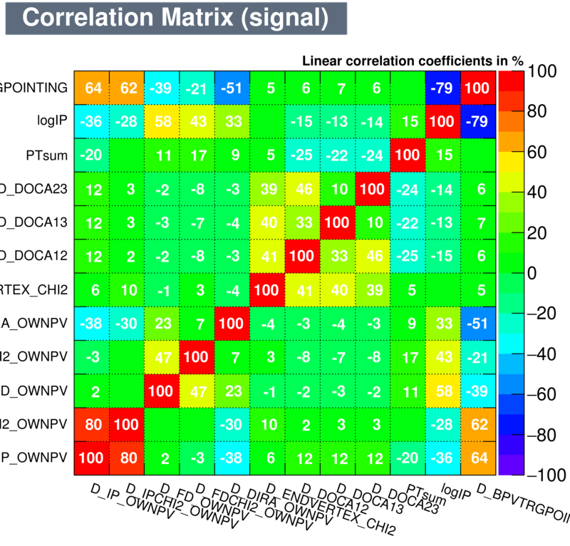
The BDTs were trained with 12 variables:
- D_IP_OWNPV
- D_IPCHI2_OWNPV
- D_FD_OWNPV
- D_FDCHI2_OWNPV
- D_DIRA_OWNPV
- D_ENDVERTEX_CHI2
- D_DOCA12
- D_DOCA12
- D_DOCA23
- PTsum
- logIP
- D_BPVTRGPOINTING.
Those variables were chosen because cut on them is have shown to have relatively small effect on the structure of the acceptance, when comparing with cutting on the kinematic variables of the daughters.
Figures below shows the variables for signal and background in the standard TMVA fashion:

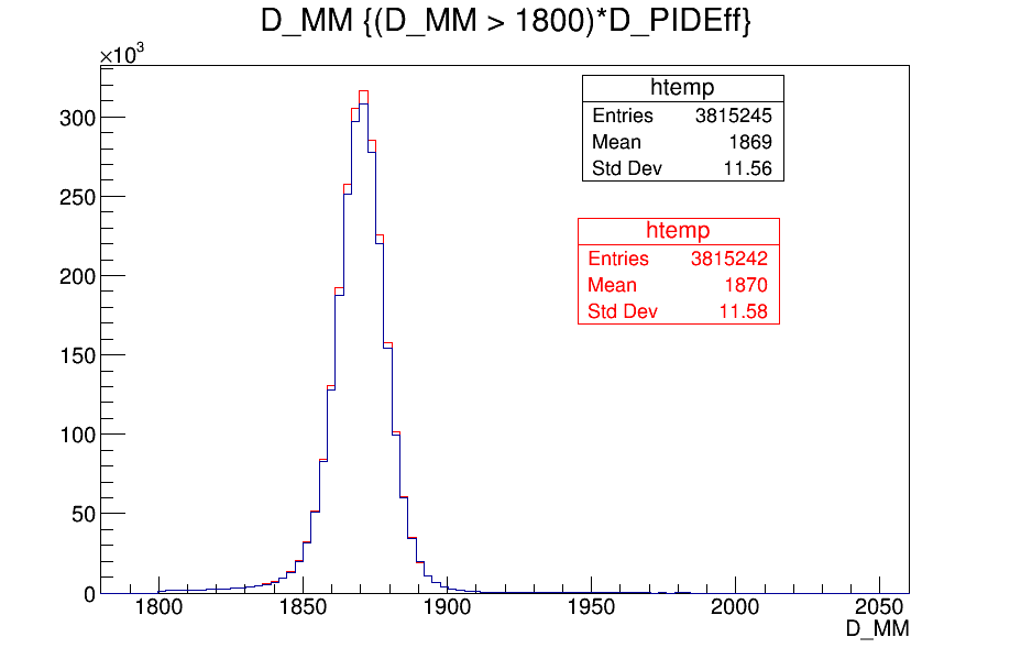
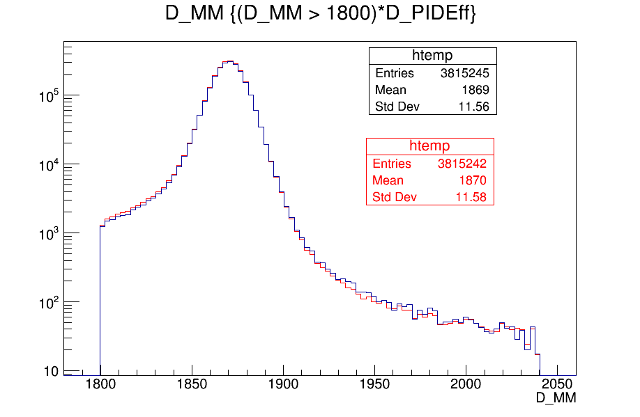
Signal mass spectrum (odd events index): red - with all weights applied but PIDeff during the training. Blue: with only PIDeff.
Background mass spectrum:
TMVA results
Below some results from the training and testing of the BDTs with the following configuration (trainning):| BDT - BDTPCA - BDTG | |
|---|---|
| Parameter | Value |
| Number of trees | 850 - 1000 - 1000 |
| MinNodeSize | 2.5% - 2.5% - 2.5% |
| MaxDepth | 3 - 3 - 2 |
| BoostType | AdaBoost - AdaBoost - Grad |
| AdaBoostBeta | 0.5 - 0.5 - none |
| Shrinkage | none - none - 0.10 |
| UseBaggedBoost | yes - yes - yes |
| BaggedSampleFraction | 0.5 - 0.5 - 0.5 |
| SeparationType | GiniIndex - GiniIndex - none |
| nCuts | 20 - 20 - 20 |
| VarTransform | none - PCA - none |
| Correlation matrix | |
|---|---|
| Signal | Background |
 |
 |
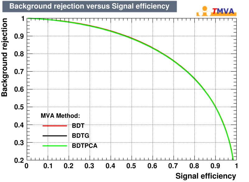
| Rejection Background vs Signal efficiency |
|---|
 |
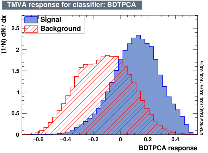
| Classifiers | |||
|---|---|---|---|
| Parameter | BDT | BDTPCA | BDTG |
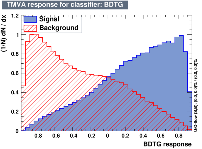
| Output | 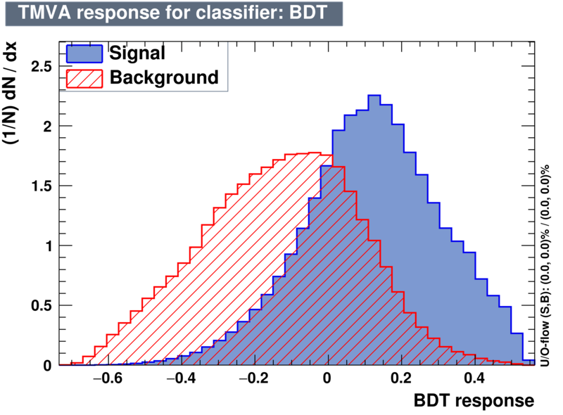 |
 |
 |
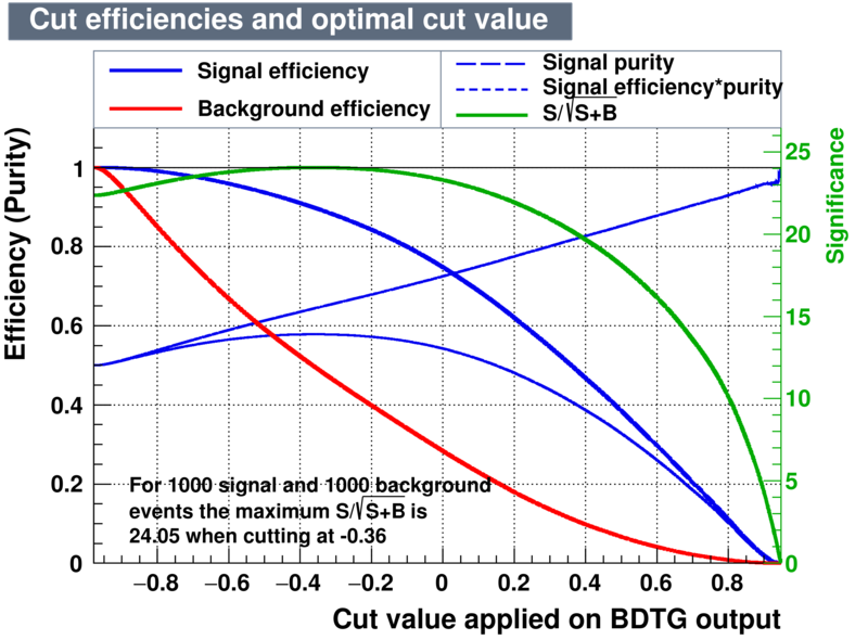
| Efficiencies | 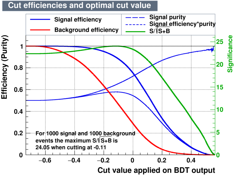 |
 |
 |
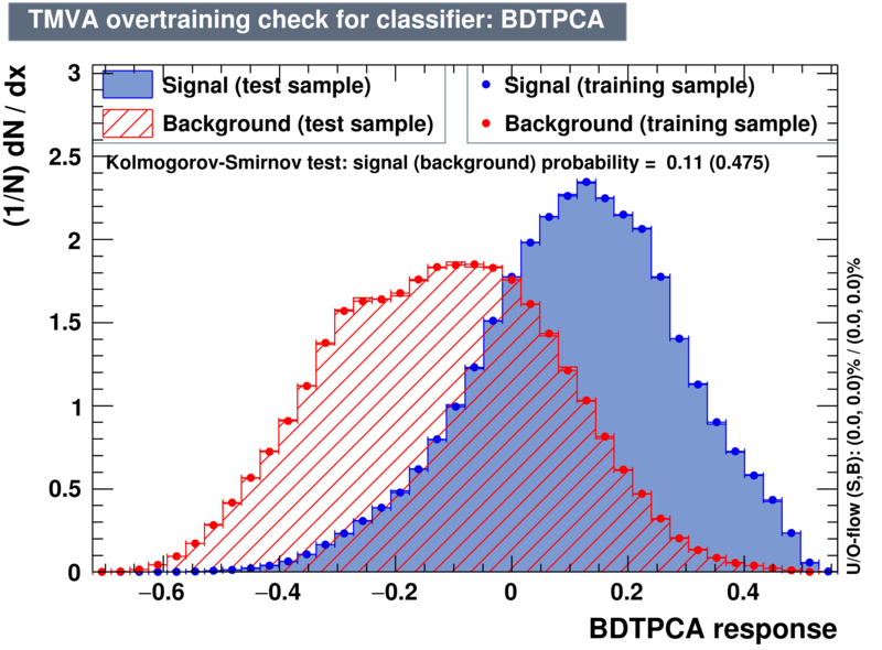
| Overtrain | 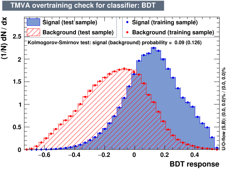 |
 |
 |
TMVA Application
By apply each classifier cut on the even selection of data, the purity and data retention can be seen on the plots below:

BDT >
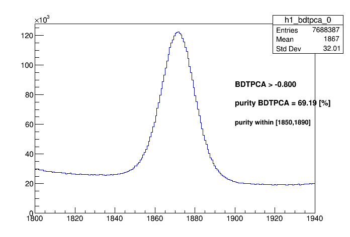
BDTPCA >
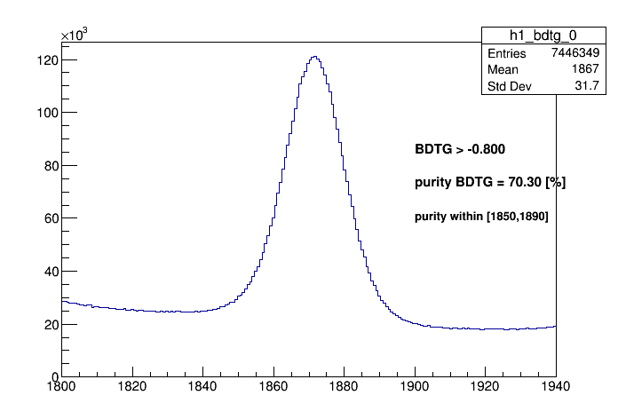
BDTG >
According to the application above one can conclude the best training interms of performance of signal retention is the BDTG. A cut of BDTG > 0.74 should have a purity of 95.22% in a windows of 1850 < D_MM < 1890 where the background was estimated from the wings of 1810 < D_MM < 1830 and 1910 < D_MM < 1930. However the yields is evaluated precisely from the fit on the mass spectrum.
Fit of the mass spectrum
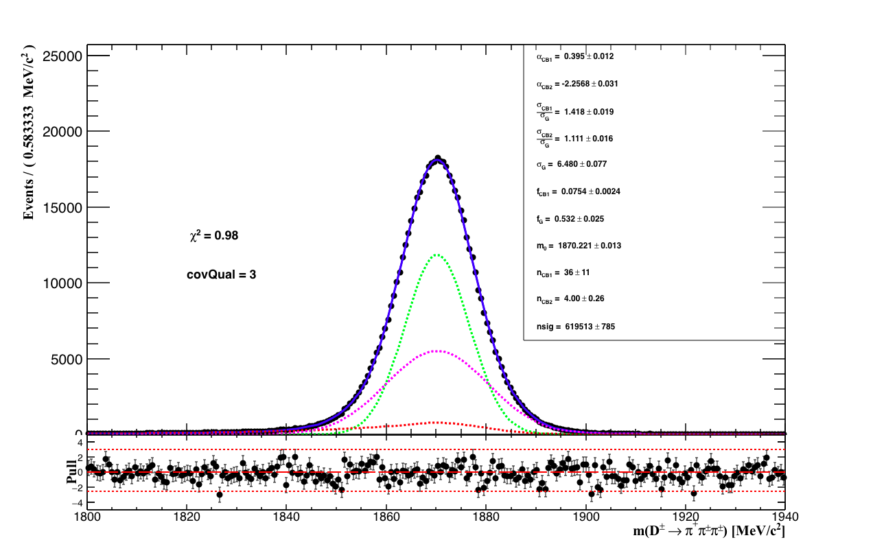
The fit to the mass spectrum is performed in two steps: first the form factor of the PDF is extracted from the fit to the MC sample. The signal PDF is composed of one Gaussian, which makes the core of the total PDF, plus two asymmetric Crystal-Balls, which make the left and right tails of the signal shape. The fit the MC sample can be seen below along with the table of the fit result.
| Fit result: D mass MC | |
|---|---|
| Parameter | Value |
| Status | RooFitResult: minimized FCN value: -5.38533e+06, estimated distance to minimum: 0.537938 covariance matrix quality: Full, accurate covariance matrix Status : MINIMIZE=0 HESSE=0 MINOS=0 |
| Floating Parameter | FinalValue ± Error |
| α1 | 0.395103 ± (-0.00471499,0.00485237) L(0.05 - 5) |
| α2 | -2.25678 ± (-0.0502108,0.0429352) L(-5 - -0.04) |
| σ1/σG | 1.41803 ± 0.0189923 L(0.7 - 20) |
| σ2/σG | 1.11134 ± (-0.023375,0.026046) L(0.7 - 20) |
| σG | 6.47984 ± (-0.0704409,0.0689378) L(6 - 15) |
| frac CB1 | 0.0753901 ± (-0.00207933,0.00176416) L(0 - 1) |
| frac G | 0.532361 ± (-0.025808,0) L(0 - 1) |
| m0 | 1870.22 ± (-0.0152029,0.0146498) L(1868 - 1871) |
| nCB1 | 35.5666 ± 11.42 L(0 - 100) |
| nCB2 | 3.99991 ± (0,0.344717) L(0 - 10) |
| nsig | 619513 ± (-791.91,782.272) L(0 - 700000) |
Click here to see the fit log
The PDFs of the figures follow the pattern: solid blue: total PDF; dashed green; Gaussian; dashed red: CB1 and dashed magenta: CB2. The black dots are the simulation of the reconstructed mass spectrum of the of the D hadron decays, where four weights were applied: ntrack correction, PID efficiency from PIDCalib, sweight from the Splot tookit evaluated from data to enhence signal and the weight of the MVA approach to correct the kinematic variables used to train the BDT. The cuts applied in the MC selection is the same that of the data selection.
The background of the signal region are dominated by combinatorial events which pass the signal selection. It is then described by a single exponential. During the fit to data, the parameters describing the tails of the CBs (α1,α2,nCB1,nCB2), the relative fraction (fracG, fracCB1) and the ratio between the width of the CBs and the with of the Gaussian (σ1/σG,σ2/σG) were set fix. Only the common mass and width of the signal PDF and the exponential slope are left to float.
The data selection is defined by the even index, with BDTG > 0.7 and cut on the pi_PIDeff > -2 (i = 1,2). The fit result is shown below:
In the figure the vertical dashed lines is the region of 2σeff where σeff = 9 MeV is the effetive width defined as
 .
And the signal region is 1853.51 < D_MM < 1889.51 MeV.
The purity (signal yield/total events) in the signal region 95.23 %. The signal yield in the region is 782319 (~93% of the total signal PDF ) events while
the total number of events in the signal region is 821081.
The table below summarizes the fit to data result.
.
And the signal region is 1853.51 < D_MM < 1889.51 MeV.
The purity (signal yield/total events) in the signal region 95.23 %. The signal yield in the region is 782319 (~93% of the total signal PDF ) events while
the total number of events in the signal region is 821081.
The table below summarizes the fit to data result.
| Fit result: D mass MC | |
|---|---|
| Parameter | Value |
| Status | RooFitResult: minimized FCN value: -8.27871e+06, estimated distance to minimum: 0.000529989 covariance matrix quality: Full, accurate covariance matrix Status : MINIMIZE=0 HESSE=0 MINOS=0 |
| Floating Parameter | FinalValue ± Error |
| αExp | -0.0050348 ± (-0.000139687,0.000134016) L(-1.12 - -1e-05) |
| m0 | 1871.51 ± (-0.0107054,0.0108042) L(1865 - 1875) |
| σG | 6.9900 ± (-0.00833704,0.00855032) L(6 - 20) |
| nComb | 134457 ± (-767.606,764.735) L(0 - 987540) |
| nsig | 843779 ± (-1022.18,1029.53) L(0 - 987540) |
Click here to see the log of the fit to data.
Efficiency
The efficiency as a function of the Dalitz plot variables is determined from the LHCb simulation. The D →πππ MC sample is generated with constant matrix element, resulting on an uniform Dalitz plot distribution.
The MC events pass through the same stages as the data (geometrical acceptance, reconstruction, stripping, full L0, Hlt1 and Hlt2 trigger requirement and MV selection) but no PID requirements are made, since the response of the RICH is not well modeled in the MC. Since the StrippingD2hhh_KKKLine stripping line has a PID cut on all kaons, the inclusive stripping is used instead.
There are known differences between the L0 simulation and the data. However, given that the D →πππ candidates are selected by the Hlt2CharmHadD2HHH line, which in turn has a requirement on the Hlt1TrackAllL0, the L0 trigger requirement needs to be made in the MC. Data-driven methods are applied to account for PID efficiency and to correct for the L0 trigger simulation. While the PIDCalib tool is used to determine the PID absolute efficiency, the L0 trigger correction is determined from the efficiency tables.
In the Dalitz plot fit, events that are L0 TOS were removed from the fit . These two L0 requirements whould have different impact on the Dalitz plot, and is should be necessary to treat each separately when computing the efficiency map for the combined sample. Therefore, we decide not to use L0 TOS events.
Two MC sample productions were habe being used in this analyses: XXXXXX sim whatever and YYYYYY sim whatever.
A histogram is filled with the weighted MC events. Since the sample of full MC was generated with a phase space distribution, the efficiency at a given position in the Dalitz plot is simply the height of the bin of the event. Bins near the border of the Dalitz plot may be only partially contained in the phase space, causing the efficiency in these bins to be artificially lower. This effect is accounted for by adding to the empty bins just at the border of the kinematic allowed region of the DP a content which is the average of the two or three neighbour bins and then, devide the weighted histogram by a histogram from a very large ToyMC sample with uniform distribution. All of this manipulation is done with, typically, a 30x30 bins histograms, but not all of the bins are occupied. In order to reduce the effect of the coarser binning of the original histogram, a smoothing process is required. A 2D cubic spline is then used to produce a high-resolution smoothed histogram, which is used in the fit. The spline procedure is based on the code LauCubicSpline from the Laura++ project.
The acceptance map is used to correct for detector efficiencies and distortion on the DP created by the selection procedures. The figure below shows the efficiency map as function of the s12 and s13 variables where the PID efficiency, Ntrack weight and the weight from the MVA approach were applied. The at the right side is the same histogram but was divided by the toyMC.
The figure below shows the efficiency map (right histogram of the above plot) after apply the smoothing spline method.
Observe at the edge of the lego plot that this procedure have a lower efficiency in kinematic limits of the signal. To account for this inefficiency extra bins is added on the edge of the efficiency histogram such that its content is the average of the content of the neighbor bins.
The effect of this correction is shown below:
Observe the flatness of the above lego histogram in comparison with the previous result, which does not have extra bins. The left histogram above is the one used to correct for selection and geometry acceptance into the fit to the Dalitz plot.
Background Model
As shown above, the background contaminating the signal region (~5% from the mass spectrum fit to data) is expected to be dominated by combinatorial events. Therefore the background model is built from data extracted from the sidebands 1810 < D_MM < 1830 MeV and 1910 < D_MM < 1910 MeV. The background model efficiency is then evaluated by the smoothing procedure as is the signal. Before the spline method be applied extra bins were applied in the border of the DP.
From the figure below one can conclude that the background from the side bands to the left and to the right of the signal region are dominated by combinatorial events.
Dalitz plot fitting
The Dalitz plot fitting is performed in order to determinine the relative phase and amplitude of each ressonances considered in the Isobar model. A PDF is defined in function of the Dalitz plot variables \(S_{12}\) and \(S_{13}\). Below is a compendium of results. We start by defining a baseline model and then systematically add more resonances until a concise model is estabilished. The figure of merit for the among models is the \(\chi^2 \) distribution as function of the DP variables and the pull distribution.
During the fit procedure the efficiency map across the Dalitz is included (see the acceptance above) and the small background contribution \(\sim 5%\). Furthermore the relative background contribution is fixed in the fit which was estimated from the fit to the mass spectrum.
Signal and Background PDF
The Dalitz plot of the \(D^{\pm}\rightarrow \pi^{\pm}\pi^{+}\pi^{-}\) events is represented by a probability density function (PDF) which consists of signal and background probability functions.
The total amplitude of the decay is: $$ A(s_{12}, s_{13}) = a_{NR}e^{i\delta_{NR}} + \sum_i a_ie^{i\delta_i}[A_i(s12,s13) + A_i(s13,s12)] $$ where \(A_i(s_{12},s_{13})\) are the dynamical amplitudes (relativistic Breit-Wigner, Polar, Gounaris-Sakurai etc...) and \(a_i\) and \(\delta_i\) are the free-parameters of the fit, magnitude and phase respectively. The amplitude is explicitly symmetrized with respect to \(s_{12}\) and \(s_{13}\) due to the two identical \(\pi^{+}\) in the final state. The Dalitz plot probability function of the signal is:, $$ P_{sig}(s_{12,s_{13}}) \sim |A(s_{12},s_{13})|^{2}. $$
The total PDF is given by the sum of those signal and background probability functions $$ P_{total}(s_{12},s_{13}) = {{P_{sig}}(s_{12},s_{13}) \over {N_{sig}}} \times \epsilon(s_{12},s_{13}) \times f_s + {P_{bkg}(m^{2}_{12},m^{2}_{13}) \over N_{bkg} }\times(1-f_s) $$ where \(f_s\) is the signal fraction, obtained from the mass fit and \(\epsilon(s_{12},s_{13})\) is the acceptance across the DP. \(N_{sig}\) and \(N_{bkg}\) is the number of signal and background events respectively and is included to guarantee that the PDFs are individually normalized. \(P_{bkg}(m^{2}_{12},m^{2}_{13})\) is the background PDF extracted from the DP of the side bands of the mass spectrum (see above).
Fit Procedure
To determine a complex amplitude in a specific model with \(N\) resonances, the data is fitted maximizing the total PDF(s12,s13) using the unbinned log-likelihood fit: $$ \mathcal{L} = \prod_i^{N} P_{i}(s_{12},s_{13}|\vec{\alpha}) $$ where \(P_{i}(s_{12},s_{13}|\vec{\alpha})\) is the PDF the resonance \(i\) and \(\vec{\alpha}\) is the vector of free-parameters given by the fit result. In the Isobar Model these parameters are the magnitudes \(a_i\) and phase \(\delta_i\) of each resonance. Furthermore it can be extended to include mass and width of ressonance or others parameters. The likelihood technique consists in finding the set of parameters \(\vec{\alpha}\) that maximizes \(\mathcal{L}\), i.e. to find the function parameters that gives the maximum value for all events. ROOT's TMINUIT pachage is used to evaluate the minimum a \(fcn\) function defined as $$ fcn = -2\ln\mathcal{L} = -2 \sum_i^{N}\ln(P_i(s_{12}, s_{13}|\vec{\alpha})). $$ where the total PDF \(P_{total}\) is normalized $$ \int \int_{DP} |P_{total}(s_{12},s_{13})|^2ds_{12}ds_{13} = 1. $$
The probability of a certain final state being formed via a particular resonance is what we call decay fraction. Fractions are obtained from the fitted amplitudes, and errors are calculated using the error matrix provided by MINUIT. For a particular resonance \(i\), the fraction \(f_i\) and its error, \(\delta f_i\), are given by: $$ f_i = {{\int ds_{1} ds_{2} |A_i|^2} \over {N_f}} = {a_i^2N_{ii} \over N_f }, $$ $$ (\delta f_i)^2 = \sum_{j,k} {\partial f_i \over \partial \alpha_j}{\partial f_i \over \partial \alpha_k} cov(\alpha_j, \alpha_k) $$ where \(N_{ii}\) and \(N_f\) are the resonance \(i\) integral and the total DP integral, respectively, and \(cov(\alpha_j, \alpha_k)\) is the error matrix.
The unbinned maximum likelihood fit is not extended, just the shape of the Dalitz plot is being fitted. The \(\rho(770)\pi\) channel is chosen as reference, with magnitude \(a_{\rho(770)\pi}\) and phase \(\delta_{\rho(770)\pi}\) set to 1 and 0, respectively.
Fit Results
Below one can find results according to the models
Model 0
This is the baselyne model with the following resonances:
- \(f_0(980) + \pi \)
- \(f01500+\pi \)
- \(3\pi_{NR} \)
- \(\rho(770)+\pi\)
- \(\rho(1450)+\pi \)
- \(f_2(1270)+\pi\)
- \(f_2(1525)+\pi\)
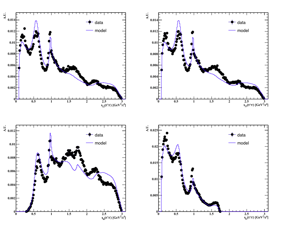
\(\chi^2\) distribution:
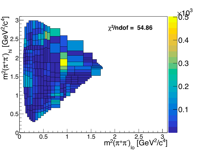
\(\chi^2\) distribution:
Projections: